Nicholas Lewis | May 10, 2020
A pdf copy of this article is available here.
Introduction
A study published in March by the COVID-19 Response Team from Imperial College (Ferguson20[1]) appears to have been largely responsible for driving government actions in the UK and, to a fair extent, in the US and some other countries. Until that report came out, the strategy of the UK government, at least, seems to have been to rely on the build up of ‘herd immunity’ to slow the growth of the epidemic and eventually cause it to peter out.
The ‘herd immunity threshold’ (HIT) can be estimated from the basic reproduction rate of the epidemic, R0 – a measure of how many people, on average, each infected individual infects. Standard simple compartmental models of epidemic growth imply that the HIT equals {1 – 1/R0}. Once the HIT is passed, the rate of new infections starts to decline, which should ensure that health systems will not thereafter be overwhelmed and makes it more practicable to take steps to eliminate the disease.
However, the Ferguson20 report estimated that relying on herd immunity would result in 81% of the UK and US populations becoming infected during the epidemic, mainly over a two-month period, based on an R0 estimate of 2.4. These figures imply that the HIT is between 50% and 60%.[2] Their report implied that health systems would be overwhelmed, resulting in far more deaths. It claimed that only draconian government interventions could prevent this occurring. Such interventions were rapidly implemented in the UK, in most states of the US, and in various other countries, via highly disruptive and restrictive enforced ‘lockdowns’.
A notable exception was Sweden, which has continued to pursue a herd immunity-based strategy, relying on relatively modest social distancing policies. The Imperial College team estimated that, after those policies were introduced in mid-March, R0 in Sweden was 2.5, with only a 2.5% probability that it was under 1.5.[3] The rapid spread of COVID-19 in the country in the second half of March suggests that R0 is unlikely to have been significantly under 2.0.[4]
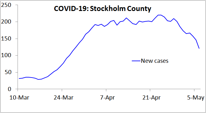
Very sensibly, the Swedish public health authority has surveyed the prevalence of individuals infected by the SARS-COV-2 virus, according to PCR testing, in Stockholm County, the earliest in Sweden hit by COVID-19. They thereby estimated that 17% of the population would have been infected by 11 April, rising to 25% by 1 May 2020.[5] Yet recorded new cases had stopped increasing by 11 April (Figure 1), as had net hospital admissions,[6] and both measures have fallen significantly since. That pattern indicates that the HIT had been reached by 11 April, at which point only 17% of the population appear to have been infected.
How can it be true that the HIT has been reached in Stockholm County with only about 17% of the population having been infected, while an R0 of 2.0 is normally taken to imply a HIT of 50%?
The importance of population inhomogeneity
A recent paper (Gomes et al.[7]) provides the answer. It shows that variation between individuals in their susceptibility to infection and their propensity to infect others can cause the HIT to be much lower than it is in a homogeneous population. Standard simple compartmental epidemic models take no account of such variability. And the model used in the Ferguson20 study, while much more complex, appears only to take into account inhomogeneity arising from a very limited set of factors – notably geographic separation from other individuals and household size – with only a modest resulting impact on the growth of the epidemic.[8] Using a compartmental model modified to take such variability into account, with co-variability between susceptibility and infectivity arguably handled in a more realistic way than by Gomes et al., I confirm their finding that the HIT is indeed reached at a much lower level than when the population is homogeneous. That would explain why the HIT appears to have been passed in Stockholm by mid April. The same seems likely to be the case in other major cities and regions that have been badly affected by COVID-19.

Figure 1. New COVID-19 cases reported in Stockholm County, Sweden, over the 7 days up to the date shown. Note that in Sweden testing for COVID-19 infection was narrowed on 12 March, to focus on people needing hospital care, so from then on only a tiny proportion of infections were recorded as cases. This would account for the lack of growth in cases during the first week plotted. Since hospitalisation usually occurs several days after symptom onset, this change also increases the lag between infection and recording as a case. Accordingly, from mid- March on the 7-day trailing average new cases figure will reflect new infections that on average occurred approximately two weeks earlier.
The epidemiological model used
Like Gomes et al., I use a simple ‘SEIR’ epidemiological model,[9] in which the population is divided into four compartments: Susceptible (uninfected), Exposed (latent: infected but not yet infectious), Infectious (typically when diseased), and Recovered (and thus immune and harmless). This is shown in Figure 2. In reality, the Recovered compartment includes people who instead die, which has the same effect on the model dynamics. The entire population starts in the Susceptible compartment, save for a tiny proportion that are transferred to the Infectious compartment to seed the epidemic. The seed infectious individuals infect Susceptible individuals, who move to the Exposed compartment. Exposed individuals gradually transfer to the Infectious compartment, on average remaining as Exposed for the chosen latent period. Infectious individuals in turn gradually transfer to the Recovered compartment, on average remaining as Infectious for the selected infectious period.
![]()
Figure 2. SEIR compartment epidemiological model diagram.
In the case of COVID-19, the diseased (symptomatic) stage is typically reached about 5 days after infection, but an infected individual starts to become infectious about 2 days earlier. I therefore set the average latent period as 3 days.[10]
The infectious period depends mainly on the delay between infectiousness and symptoms appearing and on how quickly an individual reduces contacts with others once they become symptomatic, as well as on how infectious asymptomatic cases are. In an SEIR model, the infective period can be derived by subtracting the latent period from the generation time – the mean interval between the original infection of a person and the infections that they then cause.
The Ferguson20 model assumed a generation time of 6.5 days, slightly lower than a subsequent estimate of 7.5 days.[11] I use 7 days, which is consistent with growth rates near the start of COVID-19 outbreaks.[12] The infectious period is therefore 4 (=7 − 3) days.
I set R0=2.4, the same value Ferguson20 use. On average, while an individual is in the Infectious compartment, the number of Susceptible individuals they infect is R0 × {the proportion of the population that remains in the Susceptible compartment}.
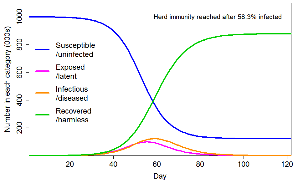
With these settings, the progression of a COVID-19 epidemic projected by a standard SEIR model, in which all individuals have identical characteristics, is as shown in Figure 3. The HIT is reached once 58% of the population has been infected, and ultimately 88% of the population become infected.
 Figure 3. Epidemic progression in an SEIR model with R0=2.4 and a homogeneous population. The time to reach the herd immunity threshold, which depends on the strength of the seeding at time zero, is arbitrary.
Modifying the basic SEIR model for variability in individual susceptibility and infectivity
The great bulk of COVID-19 transmission is thought to occur directly from symptomatic and pre-symptomatic infected individuals, with little transmission from asymptomatic cases or from the environment.[13] There is strong evidence that a small proportion of individuals account for most infections – the ‘superspreaders’.
A good measure of the dispersion of transmission – the extent to which infection happens through many spreaders or just a few – is the coefficient of variation (CV).[14] Two different estimates of this figure have been published for COVID-19. A Shenzhen-based study[15] estimated that 8.9% of cases were responsible for 80% of total infections, while a multi-country study[16] estimated that 10% were so responsible. In both cases a gamma probability distribution was assumed, as is standard for this purpose. The corresponding CV best estimates and 95% uncertainty ranges are 3.3 (3.0–5.6) and 3.1 (2.2–5.0). These figures are slightly higher than the 2.5 estimated for the 2003 epidemic of SARS.[17]
CV estimates indicate the probability of transmission of an infection. They reflect population inhomogeneity regarding individuals’ differing tendency to infect others, but it is unclear to what extent they also reflect susceptibility differences between individuals. However, since COVID-19 transmission is very largely person-to-person, much of the inhomogeneity in transmission rates will reflect how socially connected individuals are, and how close and prolonged their interactions with other individuals are. As these factors affect the probability of transmission both from and to an individual, as well as causing variation in an individual’s infectivity they should cause the same variation in their susceptibility to infection.
A common social connectivity related factor implies that an individual’s susceptibility and infectivity are positively correlated, and it is not unreasonable to assume a quite strong correlation. However, it seems unrealistic to assume, as Gomes et al. do in one case, that an individual’s infectivity is directly proportional to their personal susceptibility. (In the other case that they model, they assume that an individual’s infectivity is unrelated to their susceptibility.)
Some of the variability in the likelihood of someone infecting a susceptible individual during an interaction will undoubtedly be unrelated to social connectivity, for example the size of their viral load. Likewise, susceptibility will vary with the strength of an individual’s immune system as well as with their social connectivity. I use unit-median lognormal distributions to reflect such social-connectivity unrelated variability in infectivity and susceptibility. Their standard deviations determine the strength of the factor they represent. I model an individual’s overall infectivity as the product of their common social-connectivity related factor and their unrelated infectivity-specific factor, and calculate their overall susceptibility in a corresponding manner.[18]
I consider the cases of CV=1 and CV=2 for the common social connectivity factor that causes inhomogeneity in both susceptibility and infectivity. For unrelated lognormally-distributed inhomogeneity in susceptibility I take standard deviations of either 0.4 or 0.8, corresponding to a CV of 0.417 or 0.947 respectively. Where their gamma-distributed common factor inhomogeneity is set at 1, the resulting total inhomogeneity in susceptibility is respectively 1.17 or 1.65 when the lower or higher unrelated inhomogeneity standard deviations respectively are used; where set at 2 the resulting total inhomogeneity in susceptibility is respectively 2.17 or 2.98. The magnitude of variability in individuals’ social-connectivity unrelated infectivity-specific inhomogeneity factor does not affect the progression of an epidemic or the HIT, so for simplicity I ignore it here.[19]
Results
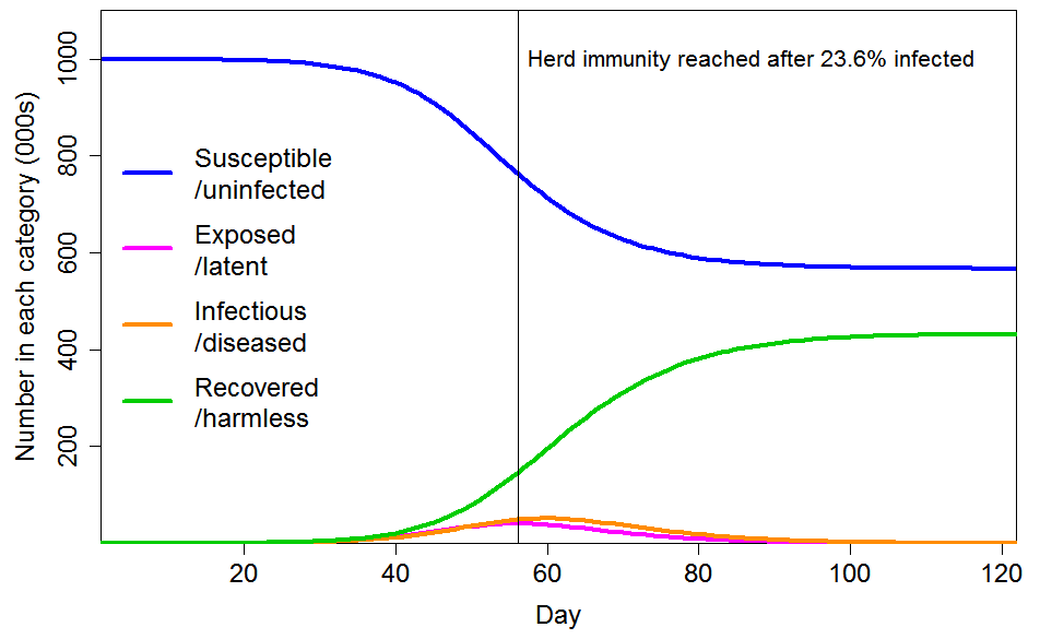
Figure 4 shows the progression of a COVID-19 epidemic in the case of CV=1 for the common social connectivity factor inhomogeneity, with unrelated inhomogeneity in susceptibility having a standard deviation of 0.4. The HIT is 60% lower than for a homogeneous population, at 23.6% rather than 58.3% of the population. And 43% rather than 88% of the population ultimately becomes infected. If the standard deviation of unrelated inhomogeneity in susceptibility is increased to 0.8, the HIT becomes 18.9%, and 35% of the population are ultimately infected.

Figure 4. Epidemic progression in an SEIR model with R0=2.4 and a population with CV=1 common factor inhomogeneity in susceptibility and infectivity and also unrelated multiplicative inhomogeneity in susceptibility with a standard deviation of 0.4.
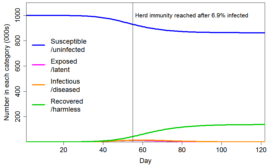
Figure 5 shows the progression of a COVID-19 epidemic in the case of CV=2 for the common social connectivity factor inhomogeneity, with unrelated inhomogeneity in susceptibility having a standard deviation of 0.8. The HIT is only 6.9% of the population, and only 14% of the population ultimately becoming infected. If the standard deviation of unrelated inhomogeneity in susceptibility is reduced to 0.4, those figures become respectively 8.6% and 17%.

Figure 5. Epidemic progression in an SEIR model with R0=2.4 and a population with CV=2 common factor inhomogeneity in susceptibility and infectivity and also unrelated multiplicative inhomogeneity in susceptibility with a standard deviation of 0.8.
Conclusions
Incorporating, in a reasonable manner, inhomogeneity in susceptibility and infectivity in a standard SEIR epidemiological model, rather than assuming a homogeneous population, causes a very major reduction in the herd immunity threshold, and also in the ultimate infection level if the epidemic thereafter follows an unconstrained path. Therefore, the number of fatalities involved in achieving herd immunity is much lower than it would otherwise be.
In my view, the true herd immunity threshold probably lies somewhere between the 7% and 24% implied by the cases illustrated in Figures 4 and 5. If it were around 17%, which evidence from Stockholm County suggests the resulting fatalities from infections prior to the HIT being reached should be a very low proportion of the population. The Stockholm infection fatality rate appears to be approximately 0.4%,[20] considerably lower than per the Verity et al.[21] estimates used in Ferguson20, with a fatality rate of under 0.1% from infections until the HIT was reached. The fatality rate to reach the HIT in less densely populated areas should be lower, because R0 is positively related to population density.[22] Accordingly, total fatalities should be well under 0.1% of the population by the time herd immunity is achieved. Although there would be subsequent further fatalities, as the epidemic shrinks it should be increasingly practicable to hasten its end by using testing and contact tracing to prevent infections spreading, and thus substantially reduce the number of further fatalities below those projected by the SEIR model in a totally unmitigated scenario.
Nicholas Lewis 10 May 2020
Update 11 May: R code used to produce the results and figures in this article is available here
Update 12 May: the reference to “prevalence of antibodies to the SARS-COV-2 virus in Stockholm County” has been corrected; it was in fact the prevalence of SARS-CoV-2 PCR-positive (infectious) individuals that was measured. This citation error has no bearing on any of the arguments made or results presented in this article.
[1] Neil M Ferguson et al., Impact of non-pharmaceutical interventions (NPIs) to reduce COVID-19 mortality and healthcare demand. Imperial College COVID-19 Response Team Report 9, 16 March 2020, https://spiral.imperial.ac.uk:8443/handle/10044/1/77482
[2] A final infection rate of 81% implies, in the context of a simple compartmental model with a fixed, homogeneous population, that the ‘effective R0‘ is between 2.0 and 2.1, and that the HIT is slightly over 50%. Ferguson20 use a more complex model, so it is not surprising that the implied effective R0 differs slightly from the basic 2.4 value that Ferguson20 state they assume.
[3] Flaxman, S. et al., Estimating the number of infections and the impact of non-pharmaceutical interventions on COVID-19 in 11 European countries. Imperial College COVID-19 Response Team Report 13, 30 March 2020, https://www.imperial.ac.uk/mrc-global-infectious-disease-analysis/covid-19/report-13-europe-npi-impact/
[4] Based on the Ferguson20 estimate of a mean generation time of 6.5 days, which appears to be in line with existing evidence, an R0 of 2.0 would result in a daily growth rate of 2.0^(1/6.5)= 11%. That is slightly lower than the peak growth rate in cases in late March in Stockholm County, and in early April in the two regions with the next highest number of cases, in both of which the epidemic took off slightly later than in Stockholm, and in line with the growth rate in Swedish COVID-19 deaths in early April
[5] https://www.folkhalsomyndigheten.se/contentassets/2da059f90b90458d8454a04955d1697f/skattning-peakdag-antal-infekterade-covid-19-utbrottet-stockholms-lan-februari-april-2020.pdf
[6] John Burn-Murdoch, Financial Times Research, 2 May 2020. http://web.archive.org/web/20200507075628/https:/twitter.com/jburnmurdoch/status/1256712090028576768
[7] Gomes, M. G. M., et al. Individual variation in susceptibility or exposure to SARS-CoV-2 lowers the herd immunity threshold. medRxiv 2 May 2020. https://www.medrxiv.org/content/10.1101/2020.04.27.20081893v1
[8] The 81% proportion of the population that Ferguson20 estimated would eventually become infected is only slightly lower than the 88% level implied by their R0 estimate of 2.4 in the case of a homogeneous population.
[9] https://en.wikipedia.org/wiki/Compartmental_models_in_epidemiology#The_SEIR_model
[10] Gomes et al. instead set the latent period slightly longer, to 4 days and treated it as a partly infectious period, unlike in the standard SEIR model.
[11] Li Q, Guan X, Wu P, et al.: Early Transmission Dynamics in Wuhan, China, of Novel Coronavirus-Infected Pneumonia. N Engl J Med. 2020; 382(13):1199–1207.https://www.nejm.org/doi/10.1056/NEJMoa2001316
[12] Once a SEIR model has passed its start up phase, and while a negligible proportion susceptible individuals have been infected, the epidemic daily growth factor is R0^(1/generation time), or 1.10–1.13 for R0=2.0–2.4 if the generation time is 7 days.
[13] L. Ferretti et al., Science 10.1126/science.abb6936 (2020).
[14] The coefficient of variation is the ratio of the standard deviation to the mean of its probability distribution. It is usual to assume a gamma distribution for infectivity, the shape parameter of which equals 1/CV2.
[15] Bi, Qifang, et al. “Epidemiology and transmission of COVID-19 in 391 cases and 1286 of their close contacts in Shenzhen, China: a retrospective cohort study.” The Lancet Infectious Diseases 27 April 2020. https://doi.org/10.1016/S1473-3099(20)30287-5
[16] Endo, Akira, et al. “Estimating the overdispersion in COVID-19 transmission using outbreak sizes outside China.” Wellcome Open Research 5.67 (2020): 67. https://wellcomeopenresearch.org/articles/5-67
[17] Lloyd-Smith, J O et al. “Superspreading and the effect of individual variation on disease emergence.” Nature 438.7066 (2005): 355-359. https://www.nature.com/articles/nature04153
[18] For computational efficiency, I divide the population into 10,000 equal sized segments with their common social connectivity factor increasing according to its assumed probability distribution, and allocate each population segment values for unrelated variability in susceptibility and infectivity randomly, according to their respective probability distributions.
[19] A highly susceptible but averagely infectious person is more likely to be removed from the susceptible pool early in an epidemic, reducing the average susceptibility of the pool. However, no such selective removal occurs for a highly infectious person of averagely susceptibility. Therefore, as Gomes et al. point out, variability in susceptibility lowers the HIT, but variability in infectivity does not do so except to the extent that it is correlated with variability in susceptibility.
[20] On 8 May 2020 reported total COVID-19 deaths in Stockholm County were 1,660, which is 0.40% of the estimated 413,000 of its population who had been infected by 11 April 2020. COVID-19 deaths reported for Stockholm County after 8 May that relate to infections by 11 April 2020 are likely to be approximately balanced by deaths reported by 8 May 2020 that related to post 11 April 2020 infections.
[21] Verity R, Okell LC, Dorigatti I, et al. Estimates of the severity of COVID-19 disease. medRxiv 13 March 2020; https://www.medrxiv.org/content/10.1101/2020.03.09.20033357v1.
[22] Similarly, the HIT may be significantly higher in areas that are very densely populated, have much less inhomogenous populations and/or are repeatedly reseeded from other areas. That would account for the high prevalence of COVID-19 infection that has been found in, for instance, some prisons and residential institutions or in city districts.


