Anthropogenic CO2 in the atmosphere per the IPCC conflicts with the observed permille values
By A. Ollila
09 March 2020
Media releases frequently news that carbon dioxide (CO2) concentration has reached a new all-time high concentration value measured in ppm. What is the nature of this CO2 increase in the atmosphere? In AR5 (p. 467), the IPCC writes: “About half of the emissions remained in the atmosphere 240 PgC±10 PgC since 1750.” The IPCC refers to Joos et al. (2001), which states that “Currently, only about half of the anthropogenic CO2 emission stays airborne.” In a newer paper of Joos et al. (2013), there is a reference to the Impulse Response Function (IRF): “The IRF is thus a first-order approximation how excess anthropogenic carbon is removed from the atmosphere by a particular model.
The carbon cycle models like Bern2.4CC and Joos et al. (2013) – which I call Joos2013 (ref. 1) in this story – show very long residence times for this anthropogenic CO2. Petteri Taalas, the Secretary-general of the World Meteorological Organization WMO, says that the residence time is over 10 000 years. Actually, it is much longer, because according to these models about 22 % of anthropogenic emissions stay forever in the atmosphere. Maybe that 10 000 years sounds more threatening creating an image that it is impossible to get rid of anthropogenic CO2 in the atmosphere. Therefore, we are doomed very soon.
The message and results of the carbon cycle models approved by the IPCC is very clear: the increased amount of the atmospheric CO2 amount from the 596 gigatons carbon (GtC) in 1750 to 866 GtC in 2017 is totally anthropogenic. You may think that of course, this increase of 270 GtC is anthropogenic due to the fossil fuel emissions totaling 433 GtC from 1750 to 2017 and the rest of emissions have gone to the ocean and to the biosphere. But it is not so.
As background information, it is needed to know that there are huge CO2 fluxes cycling between the atmosphere, the oceans, and the biosphere, Fig. 1. The yearly fossil fuel emissions are about 10 GtC and they are only about 5% of the total recycling fluxes.

Figure 1. Carbon cycle fluxes showing the yearly flux values.
I have never noticed that contrarian climate scientists have ever questioned this claim that the CO2 increase in the atmosphere is totally anthropogenic. There is a simple way to check if this is true or not.
I reckon that hardly one reader of 100 hundred readers of this website have ever heard or seen permille values. I think that the reason is the IPCC and the climate establishment. They have a skeleton if their closet and it is an essential part of the scientific climate change cheat. They follow the doctrine of the German philosopher Wittengenstein: “Whereof one cannot speak, thereof one must be silent”.
There are two permanent isotopes of carbon molecules. The most common is 12C having 6 positrons and 6 neutrons but 13C has one extra neutron. Isotope 12C is the most common being 98.9 % of all carbon and the rest is 13C. There is also a very small concentration of unstable isotope 14C, which is radioactive. Cosmic radiation produces 14C all the time by splitting nitrogen molecules in the atmosphere. Its half-life is 5730 years and it is used in radiocarbon timing method.
The measurement unit of 13C proportion (also marked as δ13C) and it is a fraction of carbon isotope 13C expressed as ‰ (written also in forms per mil, per mill, permil, permill or permille). This unit is linearly dependent on the relationship 13C/12C per eq. (1)
Permille = ((13C/12C) / (13C/12C)standard -1))*1000 (1)
This measurement unit is odd because all the values for CO2 mixtures are negative. The atmosphere is the mixture of natural CO2 and the anthropogenic CO2. The permille value of natural CO2 in the year 1750 was
-6.35‰. This value is from the research studies, which assume that in 1750 the mixing layer of the ocean and the atmosphere were in balance having the same relationship of 13C/12C. The anthropogenic CO2 means CO2 originating from fossil fuels and they have the same permille value as plants and it is -28‰. Because the permille value of fossil fuels differentiates so much from the natural permille value, it can be used for calculating the portion of anthropogenic CO2 in the atmosphere.
The permille values of the present atmosphere can be calculated by a simple equation:
Permille = ((100- CO2ant) * (-6,5) / 100 + (CO2ant) * (-28)) / 100 (2)
CO2ant is the percentage portion of anthropogenic CO2 in the atmosphere and in 2017 it was according to the IPCC = 100*270/866 = 31.2. By applying these figures, the permille value should have been -13.1‰ according to the IPCC. The measured permille value from different locations are shown in Fig. 2. The Mauna Loa value in 2017 is -8.6‰ and the error is really massive.
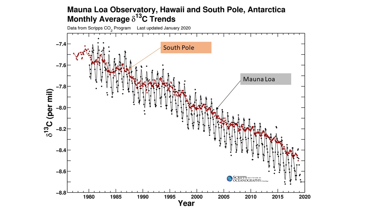
Figure 2. The observed permille values in the atmosphere.
A question may be asked that how we know that the portion of non-anthropogenic CO2 of the atmosphere has the permille value -6.5‰ nowadays. This is really a simplifying assumption because the permille value has changed a little bit due to the huge recycling fluxes. In my own model, I take this change into account. This change can happen only in one direction by decreasing the permille value of this CO2 portion because a greater permille values than -6.5‰ cannot be found in the oceans and in the biosphere. It means that the permille value calculated by a more accurate method for the present atmosphere would be slightly smaller making the error even greater.
I have pointed out that the IPCC has used research results, which are so defective, then the question is if I have a better carbon cycle model showing compliance with the observations. I do have. Recently the third version of my model by name 1DAOBM-3 has been published, ref. 2.
This model is a four-box model based on 26 physical equations. I have applied Henry’s law by assuming that the atmosphere and the mixing layer are in physical balance concerning the sequestration rate of CO2 into the ocean. In Fig. 3 the southern hemisphere ocean temperature and the CO2 concentration changes have been depicted showing the strong correlation according to Henry’s law.
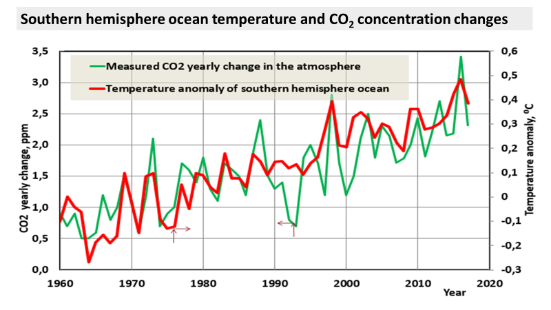
Figure 3. The southern hemisphere ocean temperature and the atmospheric CO2 concentration changes.
The most unknown factor is the sequestration rate into the deep ocean. I have used a simple linear equation. There is one parameter among the 25 equations, which is based on the empirical observations and it is the permille value of the atmosphere in 2017. Because in a recycling model you can say that “every flux depends on other fluxes”, this one empirical value determines finally the rate of anthropogenic absorption into the deep sea. The model is so much complicated that if somebody is interested in detail, he can read the paper.
I show some essential results of the simulation results of 1DAOBM-3 In Fig. 4 some calculated permille values of the models have been depicted as well as the observational values.

Figure 4. Permille values of different models and real observations.
In Fig.4 the huge error Joos2013 model can be noticed. A hypothetical value of their model is not according to the permille value definition. My model 1DAOBM-3 can calculate CO2 fluxes and amounts in reservoirs differentiating them in total CO2, anthropogenic CO2, and natural CO2 as depicted in Fig. 5, which the other models cannot do.
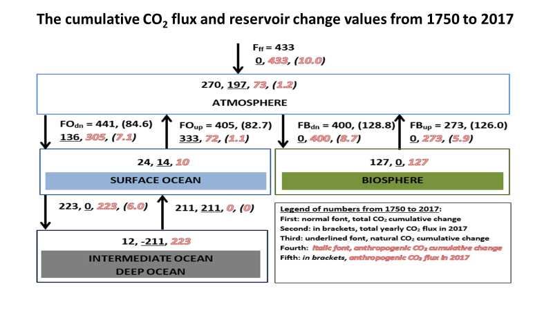
Figure 5. The cumulative CO2 flux changes and reservoir change values from 1750 to 2017.
Some major observations. The anthropogenic CO2 amount in the atmosphere in 2017 was only 73 GtC satisfying the observed permille value. The explanation is that there is natural CO2 flux from the ocean into the atmosphere bringing CO2 with non-existing or with very low anthropogenic concentration. In 2017 this flux was 1.1 GtC/yr when the same flux into the mixing layer was 7.1 GtC/yr. I think that the Joos2013 model does not recognize this fact. Because of this phenomenon, the net cumulative sequestration of the ocean in 2017 was only 36 GtC. This insignificant amount means that the sink capacity of the oceans has not utilized at all so far. The oceans have absorbed 233 GtC anthropogenic CO2. Because there were no anthropogenic CO2 in the oceans in 1750, this absorption rate has had a huge potential.
One of the major objectives of my study was to compare three carbon cycle models: my model 1DAOBM-3. Bern2.5CC, and Joos2013, which an average result of 15 different models. I did three simulations. In Fig. 6 is a scenario for CO2 emissions totaling 1000 GtC since 1750 because the known oil and gas reservoirs are about that much. The main result is that the CO2 concentration of my model stays at a lower level never reaching 500 ppm and even the other two models stay below 570 ppm.
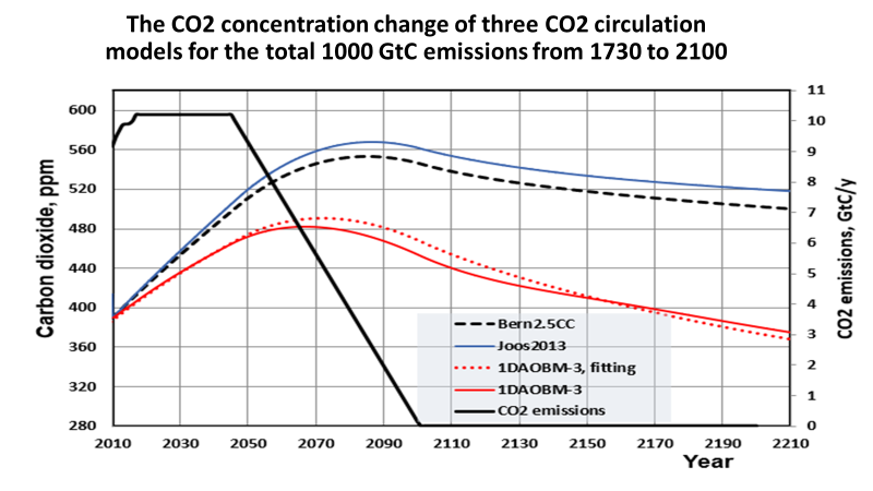
Figure 6. Simulation results of 1000 GtC scenarios for three models.
Residence times are easier to compare for impulse response. In this case, it has been assumed that the emissions would stop totally in 2010 and the models calculate what is the decay rate, in Fig. 7.
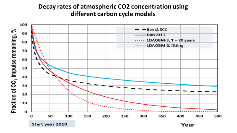
Figure 7. Decay rates for impulse response for three carbon cycle models.
This Fig. 7 shows also that the response time of my model is much shorter than the other two models. My model can be fitted using two time constants namely 12 and 150 years. From Fig.7 we can see that after 50 years the concentration would be reduced by 50 %, and in about 500…600 years the concentration would be closing zero. The other two models leave about 22 % of the initial concentration permanently in the atmosphere.
Humanity has carried out one full-scale experiment with the climate in the form of nuclear bomb tests in the atmosphere stopped in 1964. These tests produced radioactive carbon 14C. Its concentration has declined continuously, and it is closing zero as depicted in Fig. 8.
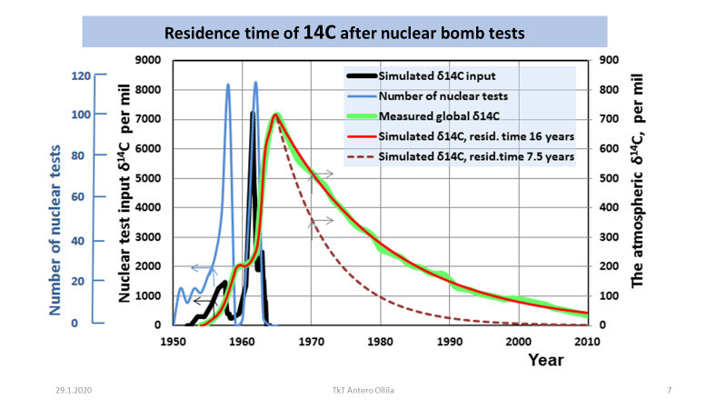
Figure 8. Radioactive carbon 14C decay rate according to the global observations.
The fitting of 16 years residence time gives almost a perfect result. This result means that the adjustment or settling time should be 4 * 16 = 64 years, which will be reached in 2028 and then only 2 % of the original concentration should be detected in the atmosphere. What this has to do with climate models? Well, this test is a perfect tracer test for the anthropogenic CO2 behavior in the atmosphere, because also anthropogenic CO2 concentration started from the zero in the system. The behavior of the total CO2 in the atmosphere is totally different, because there are huge amounts of CO2 in the recycling system and therefore its residence times is much longer for any perturbations.
There are many carbon cycle models. The most important question with any model is, how well researchers can validate their results. Validation means checking the results with real observations.
I can represent five validation results:
- The observed anthropogenic CO2 amount in the oceans in 1994 was between 118-140 GtC according to a comprehensive research study based on the deep ocean measurement,) and my model gives 123 GtC.
- The research studies about the greening of the Earth show the increase of the biomass of plants. The estimate values vary a lot with the maximum amount being 158 GtC. My model gives the value of 127 GtC in 2017.
- The residence time of the anthropogenic CO2 of my model is 16 years being exactly the same as the residence time of 14C. Compare this to the results of more than 10 000 years of Bern2.5CC and Joos2013.
- My model 1DAOBM-3 shows the coefficient of determination between the calculated CO2 and the observed CO2 to be 0.999 and the standard error 0.79 ppm. 1DAOBM-3 does not use the observed CO2 concentrations but uses the CO2 emissions and the model calculations.
- The permille value of the atmosphere follows very well the observed permille of the atmosphere, as depicted in Fig. 9.

Figure 11. The observed permille values and calculated permille values per 1DAOBM-3.
Since the error is so great (-13‰ versus -8.6‰), in which way the researchers of the papers of Joos et al. (2013) comment on this issue. Guess what. They do not comment at all. They do not calculate the permille value of the present atmosphere (the year 2011 in their paper) and they do not refer to the observed permille value as if it does not exist. It is the same thing if you have a model, which calculates the present atmospheric CO2 amount to be – let us say 1200 GtC – but then you do not calculate what is the CO2 concentration in ppm and do not comment why this number has a huge error when compared to the observed concentration. It would not work out but in the case of permille value, it seems to work, because the reviewers do not care. Why they do not care? Think about it.
I assume that the researchers of Joos el. (together 28 authors) do know that the permille value of their atmosphere is completely wrong but they want to falsify the composition of the atmosphere to show that there is so much anthropogenic CO2 and because of this very bad CO2, the humanity cannot get rid of this extra CO2 in thousands of years. Also, the huge document “Global Carbon Budget” (Ref. 3) states the increase of the atmospheric CO2 since 1750 is totally anthropogenic by nature. The climate establishment has reached such status and a position that they do not need to care about these kinds of “small” discrepancies in their science. For example, media has no idea about this cheating, and they do not believe evidence, because they do not come from Science or Nature journals but are from a well-known climate denier.
References
-
Joos, F., Roth, R., Fuglestvedt, J.S., Peters, G.P., Enting, I.G. et al., 2013. Carbon dioxide and climate impulse response functions for the computation of greenhouse gas metrics: a multi-model analysis. Atmos. Chem. Phys. 13: 2793–2825. DOI:10.5194/acp-13-2793-2013.
-
Ollila, A. Analysis of the simulation results of three carbon dioxide (CO2) cycle models. Ph. Sc. Int. Jl. 23(4), 1-19, 2020. http://www.journalpsij.com/index.php/PSIJ/article/view/30168.
-
Le Quere et al. Global Carbon Budget 2019.