Reproduction of the IPCC’s climate sensitivity gives 0.6 °C – not 1.8 °C
By Antero Ollila
March 9, 2020
The highest ranked scientific journal Nature published on the 28th of July 2016 an article based on the survey for 1,576 researchers. More than 70 % of the researchers were not able to reproduce the results of another scientist’s experiments. Are there any attempts to reproduce IPCC’s climate sensitivity?
I think that the most important key figure of the climate change science is the value of the climate sensitivity (CS), because it describes the warming effects of the major greenhouse gas carbon dioxide (CO2). CS means the temperature increase corresponding to the doubling of CO2 concentration of 280 ppm.
- IPCC’s estimates of climate sensitivity
IPCC still uses a very simple equation in calculating the global mean surface temperature response dTs (AR5, p. 664)
dTs = CSP* RF (1)
where CSP (also marked by lambda) is the Climate Sensitivity Parameter (K/(W/m2)) and RF is Radiative Forcing at the Top of the Atmosphere (TOA). IPCC says that the value of CSP is 0.5 K/(W/m2) and that it is practically constant. IPCC and many scientists as well calculate the RF value of CO2 by the equation of Myhre et al. (ref. 1):
RF = 5.35* ln(C/280) (2)
where the C is the CO2 concentration (ppm). The RF value of the CO2 concentration increase from 280 ppm to 560 ppm is 3.71 W/m2 (this value is called “the canonical estimate” by Gavin Schmidt et al. (2010)) and thus the CS = 0.5 K/(W/m2) * 3.71 W/m2 = 1.85 K. The value of TCS is between 1.0 to 2.5 Celsius degrees (later degrees) in the IPCC’s report AR5 and it means the average value 1.75 degrees (compare to 1.85 degrees). This means that the value of TCS by IPCC does not come out of blue but the equations (1) and (2) are still applicable. I limit the analysis of CS value only to this CS value, which is called transient CS (TCS) by IPCC and they say that “TCR (=TCS) is a more informative indicator of future climate than ECS” (AR5, p.111). The calculation of the equilibrium CS (ECS) by IPCC applies positive feedbacks, which are not observed so far and are therefore very theoretical. The IPCC recommends that the ECS should be used only for multi-century timescales.
- Some other estimates of climate sensitivity
There are many papers, which show lower CS than that of IPCC. I will summarize here some of them (the best estimate / the minimum estimate):
- Aldrin, 2012: 2.0 °C / 1.1 degrees
- Bengtson & Schwartz, 2012: 2.0 °C / 1.15 degrees
- Otto et al., 2013: 2.0 °C / 1.2 degrees
- Lewis, 2012: 1.6 °C / 1.2 degrees
- Lindzen and Choi, 2011: 0.7 degrees
- Idso, 1998, 0.4 degrees.
The four first studies uses IPCC’s or a GCM’s RF value without questioning it and therefore they are not real attempts to reproduce IPCC’s CS. None of these studies is based on the spectral analysis but they use the empirical temperature data. This methodology would work, if we could know the warming effects of all other warming elements like the irradiation changes of the Sun.
- Climate sensitivity parameter – CSP
I have tried to reproduce the TCS value of IPCC using the same methods as IPCC but the result is not the same. I explain the calculations in sufficient details that a reader can follow the calculation method.
The simplest method for calculation of CSP is from the energy balance of the Earth by equalizing the absorbed and emitted radiation fluxes:
SC(1-a) * (¶r2) = sT4 * (4¶r2) (3)
where SC is solar constant, a is the total albedo of the Earth, s is Stefan-Bolzmann constant, and T is the temperature (K). The total RF value for the total area of the Earth is SC(1-a)/4 and therefore eq. (3) can be written in the form
4RF = sT4 (4)
When eq. (4) is derived, it will be
d(RF)/dT = 4sT3 = 4RF/T (5)
The ratio d(RF)/dT can be inverted transforming it to CSP
dT/d(RF) = CSP = T/(4RF) = T/(SC(1-a)) (6)
The average albedo value can be calculated from the observed reflected flux and the average solar irradiation values to be 104.2 W/m2 and 342 W/m2 = 0.30468. The temperature calculated by eq. (3) is
-18.7 degrees. According to Planck’s equation, this temperature corresponds to radiation flux of 237.8 W/m2 and it is also the observed flux value emitted by the Earth into space. Theory and practise are the same, when the theory is correct. According to eq. (6), CSP is 0.268 K/(W/m2).
When Eq. (6) is written in another form it will be
T = CSP * SC(1-a) = CSP * RF (7)
There is a big difference between the CSP value of 0.5 K/(W/m2) and 0.268 K/(W/m2). The reason is well-known. The above calculations do not assume any changes in the absolute water content of the atmosphere. IPCC and the Global Climate Models (GCMs) apply calculations leading to a constant relative humidity (RH) in the atmosphere. It means that, when CO2 increases the global temperature and when the RH stays constant, the small increase of the absolute water content in the atmosphere increases the temperature. How much? IPCC writes in AR4 in section 8.6.3.1 that water vapor roughly doubles the response to forcing of GH gases and it is called positive waster feedback. In AR5 IPCC writes that water vapor’s contribution is approximately two to three times greater than that of CO2. I have checked that the doubling effect of water is technically correct because water is about 12 times stronger a GH gas than CO2 in the present climate (ref. 6) but the question is if the RH is really constant in the atmosphere.
The observed RH values measured from 1948 to 2012 are depicted in Figure 1 and they and they show that RH values are not constant.
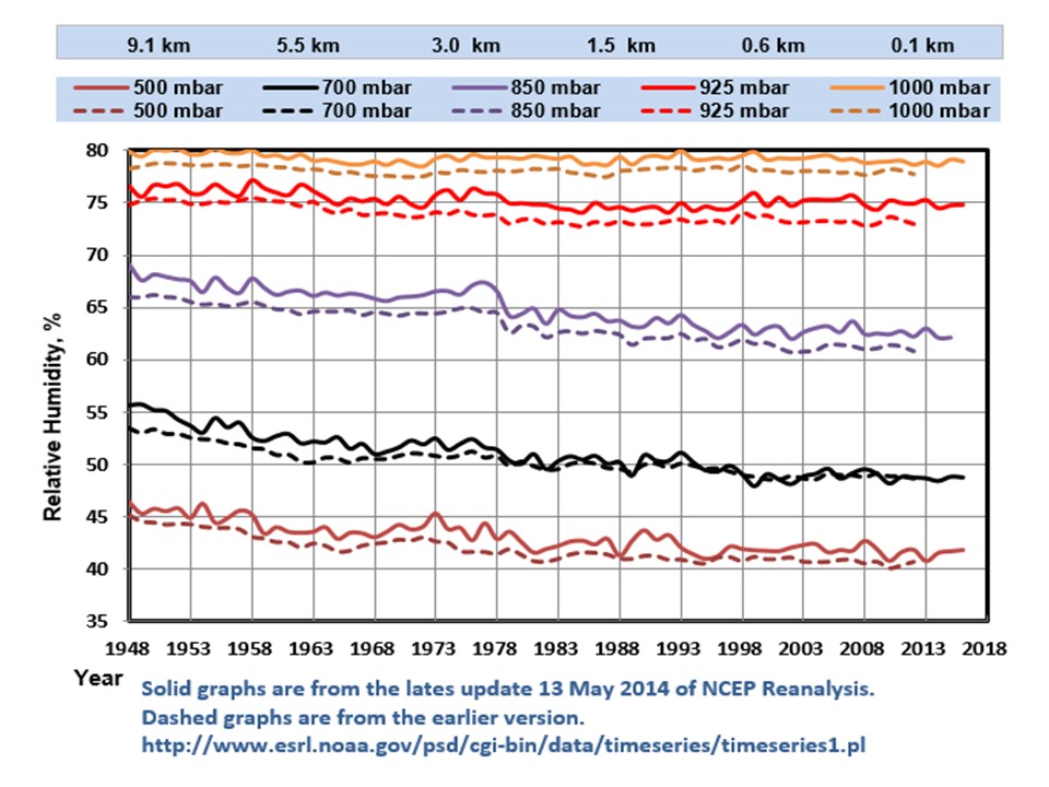
Figure 1. Relative Humidity graphs from 1948 to 2016.
It is obvious that the assumption of constant RH is not valid. Applying the CSP value of 0.268 K/(W/m2) and the RF value of 3.71 W/m2, the SC is 1.0 degrees, which is usually called Planck’s CS. As listed before, many researchers have applied different methods in calculating the CS value and a typical value is from 1.0 to 1.2 degrees. There is a good chance that these research studies have found this very same feature that there is no positive water feedback, which could double the RF value of 3.7 W/m2.
- Radiative Forcing of carbon dioxide
IPCC uses the RF formula of Myhre et al. represented in eq. (2). The formulas of Hansen et al. (ref. 2) and Shi (ref. 3) give almost the same results as one can see in Figure 2. Eq. (2) of Myhre et al. is simple and easy to use. It is a kind of standard as a measure of CO2 warming effect and it is called even “and canonical formula”.
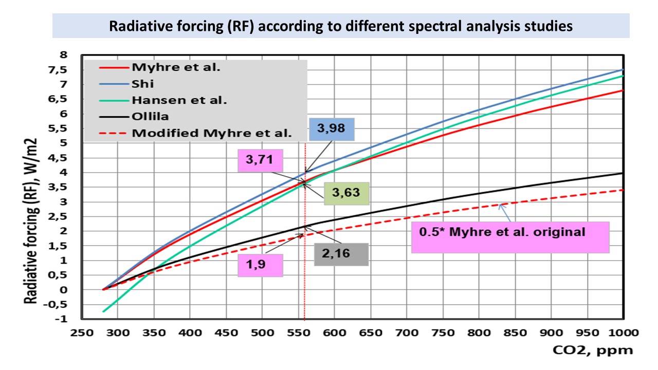
Figure 2. The RF values of CO2 according to Myhre et al., Hansen et al., Shi, and Ollila.
The first hint about the problems of this formula comes from the paper of Shi published in 1992 in journal by name “Science in China – Series B”. It is not available through network and I have received a personal electronic copy from the author himself. In Figure 3 is a print screen from a sentence, which states that the author has used a fixed RH value in his calculations. This means that the water has doubled the RF value of CO2.
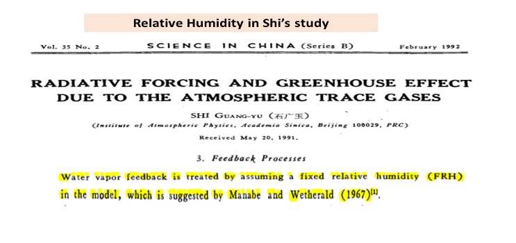
Figure 3. The RH assumption of Shi.
The only way to find out the real RF relationship is to carry out the CS calculations according to the specification of CS (ref. 4). I have used the application Spectral Calculator available through Internet and this software uses Line-By-Line (LBL) method. A very essential thing is to use the Average Global Atmosphere (AGA) profile of the Earth for the temperature, pressure and humidity. I have combined the AGA profile from the five climate zones of the Earth (available in Spectral Calculator), which has the TPW (Total Precipitated Water) value of 2.6 cm and the surface temperature of 15.0 degrees.
First I have calculated the OLR (outgoing longwave radiation) at the TOA for the CO2 concentration of 280 ppm. The OLR is the sum of emitted radiation by the atmosphere 183.8 W/m2 and the transmittance (the portion of the surface emitted radiation not absorbed by the atmosphere) 81.6 W/m2, together 265.4 W/m2. When the CO2 is increased to 560 ppm, the same radiation values are: emission 183.4 Wm2 and transmittance 79.2 Wm2, together 262.7 W/m2. Now we can see the effects of increased absorption caused by the increased concentration of CO2; the OLR has decreased as it should happen according to the theory of GH effect. Because the Earth obeys the first law of energy conservation, the ORL must increase to the original value of 265.4 W/m2. The only way this can happen, is the higher surface temperature of the Earth. By trial and error, I have found that the temperature 15.66 degrees gives emission rate of 185.0 W/m2 and transmittance of 80.4 W/m2, together 265.4 W/m2.
Because the cloudy sky calculations are not possible in Spectral Calculator, I have calculated the clear and cloudy sky values by the MODTRAN application. These results show 30 % lower OLR change than the clear sky. IPCC reports that the reduction is 25 %. Using the MODTRAN figures, the result is that the TCS value is 0.56 degrees and CSP is 0.259 K/(W/m2). The CSP value is very close to the Planck’s CSP = 0.268 K/(W/m2).
The original study of mine is published in 2014 in Development of Earth Science by title “The potency of carbon dioxide (CO2) as a Greenhouse gas” (ref. 4). My formula for the RF of CO2 is
RF = 3.12 * ln(C/280) (8)
The warming values of CO2 according to eq. (8) is depicted also in Figure 2. It is about 50 % lower than the graph of Myhre et al. In Figure 2 is also depicted a modified curve of Myhre et al. and it is done by multiplying the values of the original formula by 0.5 for eliminating the assumed water effect. This curve is fairly close to the curve depicted by eq. (8).
My CS calculations according to its specification and the text of Shi shows that the RF value of CO2 calculated by eq. (2) of Myhre et al. can be explained, if the warming effects of water are included by assuming the constant atmospheric RH conditions. There is also another possible explanation for the eq. (2). Myhre et al. have used in calculations water vapor and temperature data from the European Centre for Medium-Range Weather Forecast. This data is not publicly available and it is impossible to check what is the average global TPW value of this data.
My conclusion is that the IPCC’s warming values are about 200 % too high (1.8 degrees versus 0.6 degrees) because the CS calculation include water feedback. It is well-known that IPCC uses the water feedback in doubling the GH gas effects; even though there are relative humidity measurements showing that this assumption is not justified. CO2 radiative forcing by Myhre et al. may also include water feedback or its water content is too low.
- Validation of results
Firstly, I want to show that my spectral calculations are correct, if compared to some other published results. Kiehl & Trenberth (ref. 5) have published in 2009 an article, in which is probably the most generally used Earth’s energy balance presentation. In the LBL spectral calculations they used U.S. Standard Atmosphere 76 atmospheric profiles. They reduced the absolute water amount TWP by 12 %. Using this atmosphere, they calculated that the warming contribution of CO2 in the clear sky is 26 %; Also, this results is probably the most referred figure about the strength of CO2 as a GH gas.
I have reproduced this calculation by using Spectral Calculator and the IPCC GH effect definition, and my result is 27 % – close enough. There is only one small problem, because the water content of this atmosphere is really the atmosphere over the USA and not over the globe. The difference in the water content is great: 1.43 prcm versus 2.6 prcm. I have been really astonished about the reactions of the climate scientists about this fact. It looks like that they do not understand the effects of this choice or they do not care. Which alternative is worse? The real contribution of CO2 in using the right TWP value, and the correct GH effect definition is only 7.4 % (ref. 6).
My LBL spectral analysis is based always on the calculation of the total absorption, transmission or emission in the atmosphere. For example, the effects of GH gases are based on the variations of their concentrations. Stephens et al. (ref. 7) has summarized the results 13 of studies based on the observed values of the downward LW radiation by the atmosphere right on the surface of the Earth. The results vary from 309.2 to 326 W/m2 and the average value is 314.2 W/m2. My calculation gives the result of 310.9 W/m2, which differs 1 % from the average observed value and it is well inside the error margin of +/- 10 Wm2, which is estimated accuracy of measured LW fluxes.
References
- Myhre, G., Highwood, E.J., Shine, K.P., and Stordal, F. 1998. “New estimates of radiative forcing due to well mixed greenhouse gases.” Geophys. Res. Lett. 25, 2715-2718. http://onlinelibrary.wiley.com/doi/10.1029/98GL01908/epdf
- Hansen, J., Fung, I., Lacis, I., Rind, A., Lebedeff, D., Ruedy, S., Russell,G., and Stone, P. 1998. “Global Climate Changes as Forecast by Goddard Institute for Space Studies, Three Dimensional Model.” J. Geophys. Res., 93, 9341-9364. https://pubs.giss.nasa.gov/abs/ha02700w.html
- Shi, G-Y. 1992. “Radiative forcing and greenhouse effect due to the atmospheric trace gases.” Science in China (Series B), 35, 217-229. Not available online.
- Ollila, A. 2014. “The potency of carbon dioxide (CO2) as a greenhouse gas”. Dev. Earth Sc., 2, 20-30.
http://www.seipub.org/des/paperInfo.aspx?ID=17162 - Kielh, J.T. and Trenberth, K.E. 1997. “Earth’s Annual Global Mean Energy Budget.” Bull. Amer. Meteor. Soc. 90, 311-323. http://journals.ametsoc.org/doi/pdf/10.1175/1520-0477%281997%29078%3C0197%3AEAGMEB%3E2.0.CO%3B2.
- Ollila, A. The greenhouse effect definition. Physical Science International Journal, 23(2), 1-5, 2019
https://doi.org/10.9734/psij/2019/v23i230149
- Stephens, G.L., et al. 2012. “The global character of the flux of downward longwave radiation”. J. Clim., 25, 2329-2340. http://journals.ametsoc.org/doi/pdf/10.1175/JCLI-D-11-00262.1