
Atmospheric carbon dioxide variations at Mauna Loa Observatory, Hawaii
————————————————————–
By CHARLES D. KEELING, ROBERT B. BACASTOW, ARNOLD E. BAINBRIDGE, CARL A. EKDAHL, J R , PETER R. GUENTHER, and L E E S. WATERMAN, Scripps Institution of Oceanography, University of California at San Diego, La Jolla, California, USA and JOHN F.S. CHIN, National Oceanic and Atmospheric Administration, Mauna Loa Observatory, Hawaii
(Manuscript received February 16, 1973; in final form January 27, 1976)
ABSTRACT
The concentration of atmospheric carbon dioxide at Mauna Loa Observatory, Hawaii is reported for eight years (1964-1971) of a long term program to document the effects of the combustion of coal, petroleum, and natural gas on the distribution of CO2 in the atmosphere. The new data, when combined with earlier data, indicate that the annual average CO2 concentration rose 3.4% between 1959 and 1971. The rate of rise, however, has not been steady. In the mid-1960’s it declined. Recently it has accelerated. Similar changes in rate have been observed at the South Pole and are evidently a global phenomenon.
Introduction
In conjunction with the Antarctic study of atmospheric carbon dioxide discussed in the preceding paper (Keeling e t al., 1976), a nearly uninterrupted series of CO2 measurements has been obtained with a continuously recording nondispersive infrared gas analyzer over a period of fourteen years at the Mauna Loa high altitude observatory on the island of Hawaii. The sampled air at the station, as shown by Pales & Keeling (1965), is approximately representative of air above the North Pacific trade wind inversion between 15″ and 25″ N. Two major features of the data are a seasonal oscillation and a long term increase. The seasonal oscillation, with little doubt, reflects the integrated uptake and release of CO2 by land plants and soil (Junge & Czeplak,1968). The amplitude of the seasonal oscillation is maximum in the Arctic (Kelley, 1969) and decreases southward until low values are reached in the mid-southern hemisphere (Bolin & Keeling, 1963). The amplitude also decreases with height above ground and is barely observable in the lower stratosphere (Bolin & Bischof, 1970; Bischof, 1973). The greater amplitude in the northern hemisphere is explained by the greater extent of boreal as compared with austral forests and grasslands. The decrease with height occurs because the seasonal oscillation, produced at ground level, is progressively attenuated upward by mixing. Both the Antarctic and Mauna Loa data show an annual increase in CO2 concentration of the order of 1 ppm (parts per million of dry air). This increase reflects the retention in the air of about half of the CO2 produced by combustion of fossil fuels (Keeling, 1973). The rate of increase has not been strictly proportional to the rate of combustion of fossil fuels in either hemisphere.
Observing site
Mauna Loa Observatory is located 3400 meters above sea level on an extensive lava flow on the north slope of the largest active volcano in the Hawaiian Islands. The observing site and its meteorological milieu have been described by Price & Pales (1959), Pales & Keeling (1965), Mendonca & Iwaoka (1969), and Mendonca (1969). Some detectable CO2 emanates from volcanic sources upslope. Extensive land plants, 30 km to the east and beyond, also produce observable changes in CO2 concentration at the observatory.
Until July 21, 1967, electrical power was obtained from a local, diesel engine-driven generator. Thereafter, a transmission line has supplied municipal power. This change has nearly eliminated local production of CO2 by the station itself, but, with the completion of a paved public road to the station in July, 1969, daytime automobile pollution has become a problem.
Sampling program
Continuous measurements of atmospheric CO2 relative to dry air were made with an Applied Physics Corporation dual detector infrared analyzer, as described by Smith (1953).
This analyzer registered the concentration (mixing ratio) of CO2 in a stream of air flowing at approximately 0.5 l min-I. Every 20 min the flow was replaced for 10 min by a stream of calibrating gas called a “working reference gas”, and every few days this and additional reference gases were mutually compared to determine the instrument sensitivity and to check for possible contamination in the air handling system. These reference gases, stored in size 3A stainless steel cylinders, were themselves calibrated against specific standard gases for which the CO2 concentration had been determined manometrically, as discussed below. The experimental procedure in all essential details has remained as described by Pales & Keeling (1965).
Reference gas calibration
The concentration of atmospheric CO2 deduced from the infrared measurements at Mauna Loa depends directly on the concentration of CO2 attributed to the reference gases used to calibrate the analyzer. For this reason, considerable effort has been taken to suppress both random and systematic errors arising from use of these gases.
Each working reference gas used at the observatory in the determination of CO2 in air was routinely compared twenty or thirty times during its period of use with semipermanent standard reference gases kept at the observatory and thirty times with similar semi-permanent standards kept at the Seripps central laboratory. The comparisons at Scripps were made partially before and partially after use at the observatory to assure detection of any significant long term drift in working gas concentration. Also, the semipermanent standards held at the observatory were compared with the semipermanent standard gases at Scripps at least fifty times before and fifty times after use in the field. Certain semipermanent standards at Scripps in turn were closely compared (at least 150 times) with a special set of manometrically calibrated standard gases also kept at the Scripps laboratory.
The infrared analyzer data involved in these calibrations were obtained as pen traces on a strip chart recorder. The differences between successive traces in recorder chart ordinates were read where the trace registered a change in Concentration between the two gas mixtures being compared. All comparisons were brought to a common scale proportional to instrument response by arbitrarily assigning a magnitude to two reference gases at the beginning of the investigation in 1957. The resulting scale has been informally called the “Scripps index” scale. In 1959, a provisional manometric investigation was carried out. From this study, a linear relation between index and the mole fraction of CO2 in nitrogen was determined in the narrow range of atmospheric CO2 concentration variation where linearity in instrument response could be reasonably assumed, i.e. from approximately 310 to 330 ppm (parts per million of dry air). This approximate mole fraction scale will be designated the “adjusted CO2 index” scale because, as in the case of the previous scale, it is linearly related to instrument response.
All published data which depend on the Scripps reference gases as a basis for comparison, have, as far as we know, been expressed in the units of this adjusted index scale. Ekdahl et al. (1971) estimated that the standard deviation of an individual comparison of atmospheric CO2 concentration in air with that of a reference gas of nearly the same CO2 concentration is approximately 0.3 ppm
Table 1. Apparent downward shift in CO2 mole fraction (in ppm) as measured by applied Physics
Model 70 Infrared Analyzer when nitrogen is substituted for carrier gas as specified
| Carrier gas | ||||
| Method | Adjusted CO2 index | 79.1 % N2 20.9 % 0, |
99.07 % N2 0.93 % A |
CO2-free air |
| Analysis | 310 | 3.50 | .20a | 3.70 |
| Synthesis | 3.44 | .24 | 3.68b | |
| Analysis | 320 | 3.68 | .21a | 3.89 |
| Synthesis | 3.63 | .25 | 3.88b | |
| Analysis | 330 | 3.87 | .23a | 4.10 |
| Synthesis | 3.82 | .26 | 4.08b |
a Determined by difference.
b Determined by sum.
for the analyzer at Mauna Loa Observatory. The standard deviation for an individual comparison between two reference gases in the range 200 to 450 ppm has been found to be approximately 0.5 ppm for the analyzer at the Scripps laboratory. It follows that the daily means obtained routinely for Mauna Loa are imprecise with respect to the Scripps manometric standard gases by less than 0.1 ppm (1 standard deviation in the mean).
The inaccuracy of the manometric standard gases is more difficult to establish than the imprecision in the infrared comparisons because no procedure can prove the absence of undetected systematic errors. We have employed two related manometric methods of calibration to establish the mole fraction ofCO2 in reference gases: (1) analysis in which the CO2 from aliquots taken from a cylinder of reference gas is separated from the carrier gas using a liquid nitrogen trap freeze-out technique as described by Keeling (1958), and (2) synthesis in which CO2 is mixed with carrier gas in accurately determined proportions and the mixtures compared with reference gases by infrared analysis. The carrier gases used in these studies have included pure nitrogen, oxygen, and argon, and various proportions of oxygen in nitrogen. The analysis method has also been applied to compressed air with a correction for N,O which appears in the liquid nitrogen sublimate along with CO2 (Craig & Keeling, 1963).
Provisional manometric analyses were carried out in 1959, 1961, 1970, and 1972, and an exhaustive set of analyses was made during 1974. From these results we have established that the system of semi-permanent standard reference gases at the Scripps laboratory has drifted downward almost linearly at a rate of 0.060 ppm per year with an imprecision (1 standard deviation) in this estimate of 0.007 ppm per year. We further have found that the substitution of pure nitrogen for CO2-free dry air as the carrier gas results in a decrease in infrared analyzer response. For a gas with a concentration of 3 2 0 ppm, the decrease at sea level is equivalent to a reduction in CO2 mole fraction for air of 3.89 ppm with an imprecision of 0.04 ppm.
The apparent reduction in CO2 concentration was found, within experimental precision, to be linear with oxygen mole fraction and could be expressed as a constant factor applied to the infrared response. The effect was determined both by analysis of compressed air and reference gases containing pure nitrogen, and approximately 20, 40, and 60% oxygen in nitrogen, and by synthesis of mixtures containing pure nitrogen, oxygen, or argon. The results, after smoothing the data, are summarized in Table 1.
The carrier gas effect just discussed was found to increase with decreasing total gas pressure in the measuring cell of the infrared analyzer. Measurements in the Scripps laboratory during 1974, using compressed air and pure nitrogen as a carrier gas, indicated that an upward adjustment of the Mauna Loa data of 0.44 ppm should also be applied to the infrared data in addition to the upward adjustment appropriate to sea level. In these experiments,
Table 2. Comparison between adjusted CO2 index and CO2 mole fraction (both in ppm) based on the 1974 manometric scale for CO2 in air
| 1974 manometric scale | ||
| Adjusted CO2 index | Measurement on July 1, 1960 | Measurement on July 1, 1970 |
| At sea level | ||
| 310 | 312.50 | 313.11 |
| 320 | 322.67 | 323.29 |
| 330 | 333.05 | 333.69 |
| At elevation of Mauna Loa Observatory | ||
| 310 | 312.93 | 313.54 |
| 320 | 323.12 | 323.74 |
| 330 | 333.52 | 334.15 |
the cell pressure was controlled with a Cartesian diver manostat. This estimated pressure correction, referred to an adjusted index of 320 ppm, is imprecise to only 0.02 ppm if we assume that the effect is proportional to oxygen mole fraction in the carrier gas and we include measurements made with 40% and 60% oxygen. A second set of direct measurements were carried out at Mauna Loa Observatory using most of the same gas mixtures. These measurements indicated an adjustment of 0.37 ppm, with an imprecision of 0.07 ppm.
In summary, we have computed the mole fraction of CO2 in dry air from the infrared data by the following series of equations based principally on the manometric studies of 1974:
1. Correction for drift:
Jd = J – 1.050 + 0.060t (1)
where t denotes the time of analysis in years
since January 1, 1957, and J denotes the
adjusted CO2 index in ppm.
2. Correction for 20.9% oxygen and 0.93%
argon in the carrier gas:
Jc = J d x 1.01201 [1.003157 – 2.237 x 10⁻⁴P
-2.522 x 1O-2P2] (2)
where P is the total gas pressure in mmHg within the infrared measuring chamber, and the terms within brackets sum to unity for P = 760. For Mauna Loa Observatory we substituted for P a mean station pressure of 569.9 mmHg. For gases containing pure nitrogen as the carrier gas,
Jc = Jd.
3. Conversion to 1974 manometric mole fraction scale, X, in ppm of CO2 in dry air:
 (3)
(3)
where Co =76.582, C1=0.584910, C2 = 3.1151 x 10⁻⁴ and C3 = 7.3225 x 10⁻⁷.
A condensed form of these expressions is given by Keeling et al. (1976).
The mole fraction scale, X, is approximately 3 ppm higher then the adjusted index, J, as can be seen from Table 2.
To provide continuity with previously reported data we have expressed tabular results, Figs. 1 through 4h, and Figs. 6 through 8 in terms of adjusted CO2 index values.
Local influence on carbon dioxide concentration
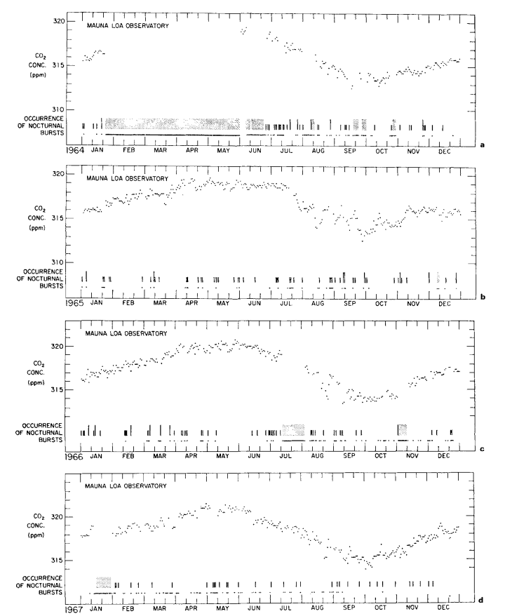
The CO2 concentration at Mauna Loa shows a persistent diurnal variation. Normally, during the night, especially after midnight, air of low humidity blows downslope. The concentration of CO2 is typically steady, but on some nights is disturbed for as much &8 several hours by irregular bursts of higher concentration. During the morning hours an Upslope wind developes, and on most days the humidity rises as moist air originally below the trade wind temperature inversion reaches the observatory. Meanwhile, the CO2 concentration typically rises for one to two hours to a “mid-day peak” and then falls until a minimum in CO2 and a maximum in humidity are reached near 1800 hr. The decline from noon maximum to afternoon minimum averages about 1 ppm; the largest decline, occurring always in summer, is about 5 ppm. Soon after 1800 hr the wind reverses direction. The CO2 concentration rises and the humidity falls until, after several hours, both attain steady values typical of night time downslope airflow.
The nocturnal bursts we attribute to the release of volcanic CO2 from a line of vents situated about 4 km upslope from the observatory. These bursts appear as highly variable recorder traces suggestive of imperfect atmospheric mixing of CO2 from a nearby source.
Fig. 1 . Hourly average atmospheric CO2 concentration at Mauna Loa Observatory versus time during the first three days of 1971. Concentrations are plotted on the adjusted CO2 index scale. Vertical bars indicate periods during which the record trace was variable, indicating local contamination. Horizontal arrows indicate periods of steady concentration. The average concentration for each steady period is indicated above the arrow.
They are routinely eliminated from further consideration in processing the data. The origin of the midday peak is less obvious.
The peak may be due in part to volcanic CO2 from some distant source downslope, but its persistence suggests a more uniform source such as vegetation. Because the dip in concentration which usually follows the peak is almost surely a result of the passage of air over the forested lower slopes during periods of photosynthetic uptake, we propose that the peak is at least in part due to the arrival of air from downslope which contains CO2 released by vegetation and soil during the previous night. Some contribution to the peak is, however, clearly from man-made sources, especially automobilies on the mountain itself. The shift from nighttime downslope to daytime upslope wind usually involves a period of light variable wind, when locally produced CO2 from combustion has maximum probability of being admitted into the sampling system.
As an example of a series of midday peaks almost surely related to automobile combustion, we show in Fig. 1 the diurnal course of CO2 at the observatory during the first three days of January 1971, when numerous visitors attended an on-site “open-house”. The afternoon dips (typically small in January) are clearly less prominent than the high midday values. The persistence of a peak is evident in the diurnal course of all data (variable traces included) for an entire month, centered on this event (Fig. 2).
From an examination of all midday peaks from 1964 to 1970, we find that 38% of those having maxima 1.5 ppm or greater than the estimated daily trend were attended by variable recorder traces, compared with 13% of those with amplitudes less than 1.5 ppm, as though the larger peaks, more often than the smaller, were associated with very local sources of CO2 but that the principal source is distant.
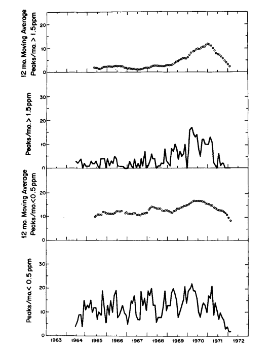
This hypothesis is also supported by comparing the long term trends in frequency of peaks having maxima greater than 1.5 ppm and less than 0.5 ppm, respectively (Fig. 3). The latter trend, except for a seasonal variation more obvious after 1966, shows only a moderate change from year to year, whereas the former shows a striking rise near the time of completion of the paved road. Still more dramatic is the decrease in frequency of large peaks after March 1971 when a locked ehain gate was erected across the road to the observatory 0.5 km from tha CO2 intakes. The smaller peaks also decreased in frequency during 1971, but more gradually. The erection of the gate happens almost to coincide with the cessation of a prolonged period of volcanic activity which commenced in November 1967 on the mountain of Kilauea. First, lava erupted for eight months in the main caldera, and then, after a short break, for twenty-three months more in the East Rift Zone. The smaller CO2 peaks at Mauna Loa are more frequent during this volcanic activity, but they are sufficiently frequent earlier to imply that enrichment by vegetation is likely to have caused most of them.
Description of data
Continuous data. Daily averages of atmospheric CO2 concentrations, based solely on steady portions of the hourly record, are plotted in Figs. 4a to 4h for 1964 to 1971. These values, which approximately reflect the CO2 in undisturbed Pacific Ocean air, were derived by the same procedure used earlier by Pales & Keeling (1965). A minor association with regional weather patterns is suggested by short period oscillations of the daily averages, but the principal feature is a seasonal oscillation which repeats with remarkable regularity from year to year. This latter oscillation shows up clearly in monthly averages of the daily values as plotted in Fig. 5, and listed in Table 3.
Table 3. Monthly average concentration of atmospheric carbon dioxide (ppm) at Mauna Loa Observatory
based on steady sub
| 1964 | 1965 | 1966 | 1967 | 1968 | ||||||
| Month | No. of days | Adjusted CO2 index | No. of days | Adjusted CO2 index | No. of days | Adjusted CO2 index | No. of days | Adjusted CO2 index | No. of days | Adjusted CO2 index |
| January | 18 | 316.13 | 26 | 316.25 | 31 | 316.84 | 11 | 318.13 | 30 | 318.60 |
| February | 316.67a | 27 | 317.32 | 27 | 317.82 | 20 | 318.54 | 28 | 319.16 | |
| March | 317.13a | 29 | 3 17.80 | 23 | 318.69 | 20 | 318.99 | 26 | 319.91 | |
| April | 318.34a | 25 | 318.92 | 23 | 319.83 | 20 | 320.45 | 25 | 320.89 | |
| May | 318.93a | 28 | 318.96 | 29 | 320.08 | 18 | 320.89 | 28 | 321.46 | |
| June | 9 | 318.86 | 29 | 318.80 | 29 | 319.81 | 23 | 319.91 | 22 | 321.40 |
| July | 20 | 317.20 | 23 | 318.15 | 9 | 318.90 | 25 | 318.67 | 30 | 320.00 |
| August | 14 | 315.23 | 24 | 315.80 | 18 | 316.31 | 24 | 317.09 | 21 | 317.98 |
| September | 14 | 313.90 | 25 | 314.68 | 21 | 314.52 | 27 | 315.46 | 30 | 316.57 |
| October | 23 | 313.78 | 30 | 314.39 | 23 | 314.17 | 30 | 315.36 | 28 | 316.27 |
| November | 28 | 314.58 | 30 | 315.81 | 16 | 315.95 | 30 | 316.7528 | 28 | 317.17 |
| December | 29 | 315.50 | 27 | 315.92 | 23 | 317.07 | 31 | 318.06 | 25 | 318.65 |
a Estimated from oscillating power function (eq.(3)).
In Table 4, column 2, are listed annual values of the steady data expressed on the adjusted CO2 index scale. In column 3 of the same table are shown averages of the full data excepting only those values (about 4 % of the total) which were evidently contaminated locally as shown by variable recorder traces. The full data (which we have also examined on a daily and monthly basis) hardly differ from the steady data because low values during afternoon dips tend to cancel with high values during midday peaks. Additional columns show the data re-expressed as CO2 mole fractions.
Supplementary data. The individual reference gas calibrations and daily average atmospheric air measurements are too extensive to reproduce here. Those for 1964 through 1970 have been summarized in a detailed report (Ekdahl et al., 1971) and deposited with the National Auxiliary Publications Service of the American Society for Information Science.1 All relevant calculations and supporting data are reported. A similar report of the measurements for 1971 will be prepared in conjunction with a subsequent article.
| 1969 | 1970 | 1971 | |||
| No. of days | Adjusted CO2 index | No. of days | Adjusted CO2 index | No. of days | Adjusted CO2 index |
| 29 | 320.08 | 31 | 321.16 | 29 | 322.60 |
| 22 | 320.85 | 27 | 322.03 | 28 | 323.05 |
| 30 | 321.90 | 31 | 323.03 | 29 | 323.65 |
| 28 | 322.82 | 30 | 324.20 | 28 | 324.29 |
| 28 | 323.45 | 27 | 324.09 | 30 | 325.51 |
| 24 | 322.76 | 28 | 323.90 | 29 | 325.06 |
| 26 | 321.89 | 28 | 322.61 | 25 | 323.93 |
| 27 | 319.61 | 20 | 321.14 | 23 | 322.12 |
| 25 | 318.56 | 21 | 319.75 | 27 | 320.24 |
| 31 | 318.03 | 25 | 319.75 | 25 | 320.37 |
| 30 | 318.94 | 26 | 320.56 | 30 | 321.60 |
| 31 | 320.35 | 27 | 321.57 | 31 | 322.70 |
Table 4. Seasonally adjusted concentration of atmospheric CO2 (in ppm) at Mauna Loa Observatory
| Adjusted CO2 index | CO, mole fraction | |||
| Year
(1) |
Annual averagea of steady data
(2) |
Annual average of full data
(3) |
Annual average of steady data
(4) |
From trend equationb
(5) |
| 1958 | Incomplete | |||
| 1959 | 313.23 | — | 316.14 | 316.30 |
| 1960 | 314.04 | — | 317.03 | 317.06 |
| 1961 | 314.66 | — | 317.71 | 317.74 |
| 1962 | 315.43 | — | 318.57 | 318.37 |
| 1963 | 315.83 | — | 319.03 | 318.98 |
| 1964 | 316.35c | — | 319.63c | 319.60 |
| 1965 | 316.90 | 316.92 | 320.25 | 320.27 |
| 1966 | 317.50 | 317.60 | 320.92 | 321.02 |
| 1967 | 318.19 | 318.14 | 321.70 | 321.88 |
| 1968 | 318.99 | 318.92 | 322.58 | 322.88 |
| 1969 | 320.71 | 320.85 | 324.47 | 324.06 |
| 1970 | 321.98 | 322.20 | 325.79 | 325.45 |
| 1971 | 322.93 | 322.94 | 326.83 | 327.08 |
a Annual averages for 1959 to 1963 are derived from Table 1 of Pales & Keeling (1965), for 1964 to 1971 from Table 3 of this paper.
b Smoothed values of steady data, for 1 July of each year, as derived from the last four terms of eq. a (6).
c Partially estimated according to values listed in Table 3.
Secular increase in CO2
Two methods have been employed to separate the annual increase of about 0.8 ppm from the 6 ppm seasonal variation found in the Mauna Loa record. In the first method, monthly average adjusted CO2 index values were fit to a function in time containing both a power series and Fourier harmonic terms. The harmonic frequencies were established by spectral analysis of the daily averages. The second method filtered out the dominant harmonic terms with a moving average.
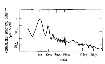
In the first approach the dominant frequencies in the daily average record of steady data from June 1964 through June 1971 were estimated from a discrete Fourier transform using the transform algorithm of Cooley & Tukey (1965). Transform terms were weighted to correspond to the cosine bell data window of Hann (Blackman & Tukey, 1959, pp. 14-15, 98; Hinnich & Clay, 1968), and afterwards converted to a power spectrum. Since the algorithm requires 2N equally spaced data, days with no data were assigned values by linear interpolation of contiguous data, and spectra were obtained from both the first and last 2048 of the 2587 data points. The average of these two spectra is shown in Fig. 6. Since days without data are unclustered (see Figs. 4a through 4h) and constitute only 17% of the record, errors from interpolation have little effect on the analysis. The only significant harmonic contributions to the long term data record are the fundamental annual cycle and its first (6 months) harmonic.
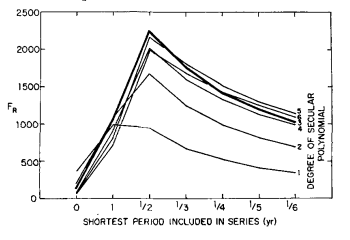
To verify that very little information is contained in higher harmonics, monthly averages of the adjusted CO2 index values were fit by the method of least squares to several trial functions consisting of power series of varying degree combined with a varying number of harmonic terms. For a given power series polynomial, the significance of the fundamental cyclic variation in combination with higher cyclic variations of 1/2 year, 1/3 year, 1/4 year, etc. was tested with the function:
FR = (R2n)/[(l – R2 ) / ( N – n – 1 ) ] (4)
where R, the multiple correlation coefficient, tends toward unity as the “goodness of fit” increases; n is the number of parameters determined by the least squares fit; and N is the number of data. The statistic FR, which follows the F distribution (Bevington, 1969, p. 199), was found to be maximized when only the fundamental and its first harmonic were included in the trial function (Fig. 7). Also, FR was maximized when the secular trend included powers of time up through the third.
Accordingly, the monthly average adjusted CO2 index values were corrected to the CO2 mole fraction scale and then fit with the function:
(5)
X(t) = Q1 sin 2πt + Q2 cos 2πt + Q s sin 4πt
+Q4 cos 4πt + Q5 + Q 6 t + C7t2 + Q8t3
where X denotes the CO2 mole fraction of dry air in ppm, t is the elapsed time, in years, relative to the first of January, 1958, and
(6)
Q2 = -1.065 ppm
Q3 = -0.343
Q4 = 0.583 ppm
Q6= 1.213 ppm/yr
Q7 = -0.100 ppm/yr2
Q8 = 0.00545 ppm/yr3
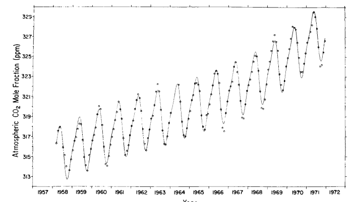
The standard deviation of the monthly averages with respect to this function is 0.27 ppm. The secular trend, which we seek, is given by the last four terms of eq. (6), as shown by the curve in Fig. 8. Values of the trend for 1 July of each year are listed on the mole fraction scale in Table 4, column 5. The relative increase in concentration from 1959 to 1971 is 3.4%.
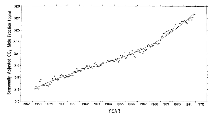
Fig. 8. Secular trend of atmospheric CO2 mole fraction at Mauna Loa Observatory, based on a cubic trend function. Circles denote seasonally adjusted monthly averages. Concentrations are expressed as the CO2 mole fraction of dry air in ppm.
This increase agrees closely with 3.1% found for the South Pole for the same time interval (Keeling et al., 1976). To provide an independent estimate of the secular trend, the monthly averages were filtered with a simple twelve months moving average (Fig. 9) as was done by Pales & Keeling (1965).
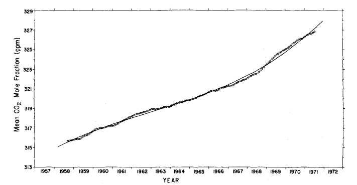
Fig. 9. Twelve month moving average of atmospheric CO2 mole fraction at Mauna Loa Observatory. Circles: means plotted versus the seventh month of the appropriate 12 month interval. Crosses: means which include concentration estimates calculated from the oscillating power function for the period February, 1964 through May, 1964. Full curve: secular trend based on cubic trend function.
We have examined the extent to which this moving average distorts the long term trend by computing its continuous analogue for the cubic trend function. Using the parameters Q5 to Q 8 of eq. (6), the maximum error, incurred at the end of the record, is entirely negligible (less than 0.02 ppm).
As already noted by Pales & Keeling (1965) for the period before 1964, the moving average suggests a weak two year cycle. The data record is of insufficient length to expect such a cycle to be evident in a spectral analysis (Fig. 6), but the possibility was tested for using the P, statistic described above. We found that no subharmonic of the annual cycle ( 2 to 6 years were tested) possesses a large enough signal to noise level to render it detectable. The moving average filter removes completely the one year cycle and its harmonics from the estimate of the secular trend. Other variability within any year of record is also attenuated, but random variations which persist over several months, such as unusually low summer or high winter means, are only moderately attenuated. In contrast, the cubic trend function (last four terms of eq. (6)) greatly attenuates not only the two dominant frequencies, but also all random variations with periods less than approximately 10 years; it thus produces a smoother estimate of the secular trend than does the moving average. Furthermore, the trend for all years is changed each time the length of record is altered, for example, by the accession of new data. At the other extreme, the succession of seasonally adjusted monthly averages (circles in Fig. 8) indicate the secular trend without suppressing any frequencies except the two dominant ones.
The data could, of course, be reprocessed using still other filters, but salient features are almost surely revealed using the three filters just discussed. The three versions of the trend so obtained have one striking feature in common: An apparent decline in the rate of in- crease of CO2 during the early 1960’s, followed by an increasing rate after 1967. Confronted with the break in record in 1964, we are reluctant to rule out the possibility that the decline is a t least partly an instrumental artifact. Unfortunately, no second record of atmospheric CO2 concentrations in the northern hemisphere exists which can help us decide whether this decline is real or not. A possible slower rate of increase is not inconsistent with data of Bolin & Bischof (1970) based on aircraft samples collected over a broad region of the polar northern hemisphere, but as these authors point out, the irregularities of their sampling schedule (see their Table 2, p, 433) “hardly permit a search for possible secular variations in the annual increase”.
If we disregard the temporary decline in rate during the early 1960’s, the change in rate roughly approximates that of fossil fuel combustion which was 60% higher in 1971 than in 1959.
Conclusions
In extending the previously published five year record of atmospheric CO2 concentrations at Mauna Loa Observatory by eight additional years, new features of CO2 in air near the Hawaiian Islands are revealed, and previously noted features more precisely defined. Statistical analysis of daily and monthly averages of the original continuous data establish a seasonal oscillation described by annual and semiannual harmonic oscillations about a long term trend. This latter trend, obtained by subtracting the average seasonal oscillation from each of the original 14 years of record, is a rising function of time and is described, within the precision of the data, by either a cubic power series, a 12 month moving average, or a set of seasonally adjusted monthly averages.
The air at Mauna Loa Observatory may be slightly influenced by local processes which cannot be expunged from the record, but the observed long term trend of rising CO2 appears clearly to be in response to increasing amounts of industrial CO2 in the air on a global scale. We are thus convinced of the observatory’s suitability to monitor global changes in atmospheric CO2 concentration.
Acknowledgements
All members of the staff of the Mauna Loa Observatory contributed to maintaining this long term program. We especially thank Mr Howard Ellis, Dr Lothar Ruhnke, and Dr Rudolf Pueschel, successive directors of the observatory, and Dr Lester Machta of the National Oceanographic and Atmospheric Administration who has guided the destiny of the station through the years of this report. We gratefully dedicate this paper to the late Mr Jack Pales who, by great personal effort, established the observatory as an environmental facility of world-wide significance.
Financial support was by the Atmospheric Sciences Program of the U.S. National Science Foundation under grants 0-19168, GP-4193, GA-873, GA-13645, GA-13839, and GA-31324X. Station facilities, field transport, and staff assistance were provided by the National Oceanographic and Atmospheric Administration, and its predecessor, ESSA.
REFERENCES
Bevington, P. R. 1969. Data reduction and error analysis for the physical sciences. McGraw-Hill, New York, 336 pp.
Bischof, W. 1973. Carbon dioxide concentration in the upper troposphere and lower stratosphere. III. Tellus 25. 305-308.
Blackman, R. B. & Tukey, J. W. 1958. The measurement of power spectra. Dover Publications, New York, 190 pp.
Bolin, 13. & Bischof, W. 1970. Variations of the carbon dioxide content of the atmosphere in the northern hemisphere. Tellus 22, 431-442.
Bolin, B. & Keeling, C. D. 1963. Large-scale atmospheric mixing as deduced from the seasonal and meridional variations of carbon dioxide. J. Geophys. Res. 68, 3899-3920.
Cooley, J. W. & Tukey, J. W. 1965. An algorithm for the machine calculation of complex Fourier series. Math. Comput. 19, 297-301.
Craig, H. & Keeling, C. D. 1963. The effects of atmospheric N,O on the measured isotopic composition of atmospheric CO2. Geochim. et Cosmochim. Acta 27, 549-551.
Ekdahl, C. A., Jr, Guenther, P. R. & Keeling, C. D. 1971. Mauna Loa carbon dioxide project, Report 4 , 349 pp. Scripps Institution of Oceanography, La Jolla, California 92037.
Hinnich, M. J. & Clay, C. S. 1968. The application of the discrete Fourier transform in the estimation of power spectra, coherence, and bispectra of geophysical data. Reviews of Geophys. 6, 347-363.
Junge, C. E. & Czeplak, G. 1968. Some aspects of the seasonal variation of carbon dioxide and ozone. Tellus 20. 422-434.
Keeling, C. D. 1958. The concentration and isotopic abundance of atmospheric carbon dioxide in rural areas. Geochim. et Cosmochim. Acta 13, 322-334.
Keeling, C. D. 1973. Industrial production of carbon dioxide from fossil fuels and limestone. Tellus 25, 174-198.
Keeling, C . D., Harris, T. B. & Wilkins, E. M. 1968. The concentration of atmospheric carbon dioxide at 500 and 700 millibars. J. Geophys. Res. 73, 451 1-4528.
Keeling, C. D., Adams, J. A. Jr, Ekdahl, C. A. Jr & Guenther, P. R. 1976. Atmospheric carbon dioxide variations at the South Pole. Tellus 28, 552-564.
Kelley, J. J., Jr. 1969. An analysis of carbon dioxide in the Arctic atmosphere near Pt. Barrow, Alaska, 1961 to 1967. Scientific Report, Office of Naval Research, Contract N00014-67-A-01030-0007, University of Washington.
Mendonca, B. G. 1969. Local wind circulation OR the slopes of Mauna Loa. J. Appl . Meteo. 8, 533-541.
Mendonca, B. G. & Iwaoka, W. T. 1969. The trade wind inversion on the slopes of Mauna Loa, Hawaii, J. Appl. Meteo. 8, 213-219.
Pales, J. C. & Keeling, C. D. 1965. The concentration of atmospheric carbon dioxide in Hawaii, J . Geophys. Res. 70, 6053-6076.
Price, S. & Pales, J. C. 1959. The Mauna Loa high-altitude observatory. Monthly Weather Rev. 87, 1-14.
Smith, V. N. 1963. A recording infrared analyser. Instruments 26, 421-427.
_____________________________________________
1 This information has been deposited with ASIS as NAPS document no. 02890. Order from ASIS-NAPS, c/o Microfiche Publications, 440 Park Avenue South, New York, New York 10016. Remit in advance for each NAPS accession number. Make check payable to Microfiche Publications. Photo-copies are $87.25. Microfiches are $3.00. Outside the United States and Canada, postage is $4.00 for a photocopy or $1.00 for a fiche.