CLIMATE SCIENTIST EXPLAINS THE AIRBORNE FRACTION
tambonthongchai.com | Dec. 29, 2020
THIS POST IS A CRITICAL REVIEW OF A LECTURE ON CARBON BUDGETS FOR THE CLIMATE ACTION OF REDUCING AND ELIMINATING FOSSIL FUEL EMISSIONS SO THAT HUMANS CAN CONTROL THE CLIMATE AND SAVE THE PLANET. LINK TO SOURCE: https://futureoflife.org/2019/10/29/not-cool-ep-18-glen-peters-on-the-carbon-budget-and-global-carbon-emissions/
PART-1: WHAT CLIMATE SCIENTIST DR. GLEN PETERS SAYS
GLEN PETERS, CLIMATE SCIENTIST, AND CARBON BUDGET EXPERT. Topic: We’ll learn what the carbon budget is and why it’s hard to calculate, why some causes of carbon emissions are harder to address than others, how the phrase “carbon footprint” is so often misused and why it’s also hard to calculate, how responsibility for emissions is attributed to different countries. Glen Peters is a Research Director at the CICERO, the Center for International Climate Research in Oslo. Most of his research is on past, current, and future trends in energy consumption and greenhouse gas emissions. He studies human drivers of global change, the global carbon cycle, bioenergy, scenarios, sustainable consumption, international trade and climate policy, and emission metrics. THE LECTURE WAS GIVEN IN A QUESTION AND ANSWER FORMAT AND IS PRESENTED IN THAT FORMAT BELOW.
QUESTION: WHAT IS THE GLOBAL CARBON BUDGET? ANSWER: In the global carbon budget, we try and look at all the sources of carbon into the atmosphere and the sort of sinks of carbon and try and understand where carbon is going. You could think about it a bit like a bathtub, where you try and look what’s going into the bathtub and see what’s going out of the bathtub and make sure they match. The carbon budget generally has two components: the source component, so what’s going into the atmosphere; and the sink component, so the components which are more or less going out of the atmosphere. So in terms of sources, we have fossil fuel emissions; so we dig up coal, oil, and gas and burn them and emit CO2. We have cement, which is a chemical reaction, which emits CO2. That’s sort of one important component on the source side. We also have land use change, so deforestation. We’re chopping down a lot of trees, burning them, using the wood products and so on. And then on the other side of the equation, sort of the sink side, we have some carbon coming back out in a sense to the atmosphere. So the land sucks up about 25% of the carbon that we put into the atmosphere and the ocean sucks up about 25%. So for every ton we put into the atmosphere, then only about half a ton of CO2 remains in the atmosphere. So in a sense, the oceans and the land are cleaning up half of our mess, if you like. The other half just stays in the atmosphere. Half a ton stays in the atmosphere; the other half is cleaned up. It’s that carbon that stays in the atmosphere which is causing climate change and temperature increases and changes in precipitation and so on. This 50% is a pretty robust number, and this is one of the great mysteries of the carbon cycle. Mystery is not really the right word, but it’s quite curious that no matter how much we’re putting in the atmosphere, this fraction that stays in the atmosphere, about 50%, has remained relatively constant. So if we go back 50 years in time for example, we still had about 50% stay in the atmosphere. Today when we emit, there’s about 50% that stays in the atmosphere, but then there’s a question of will this continue forever if we start to see the impacts of climate change — changing precipitation, maybe for example the land sink is not as good, so maybe tropical forests don’t take up as much carbon. Then we may see this share drop and more stay in the atmosphere. We know — there is some evidence that it may change, so when there’s an El Nino and it causes hotter and drier weather in the tropics, less carbon is taken up by the forests, and so we see a greater increase in the atmosphere. This is sort of natural variability, but this natural variability gives us an idea of what may happen if temperatures increase.
QUESTION: WHAT IS THE CARBON BUDGET IMBALANCE ISSUE IN CLIMATE SCIENCE? HOW DOES THAT RELATE TO WHAT YOU JUST SAID? ANSWER: The carbon budget is like a balance, so you have something coming in and something going out, and in a sense by mass balance, they have to equal. So if we go out and we take an estimate of how much carbon have we emitted by burning fossil fuels or by chopping down forests and we try and estimate how much carbon has gone into the ocean or the land, then we can measure quite well how much carbon is in the atmosphere. So we can add all those measurements together and then we can compare the two totals — they should equal. But they don’t equal. And this is sort of part of the science, if we overestimated emissions or if we over or underestimated the strength of the land sink or the oceans or something like that. And we can also cross check with what our models say. So this carbon imbalance is basically the balance between what we think is happening and whether those two things agree. And they don’t, but the good thing is that sometimes we overestimate the balance, sometimes we underestimate it — which means that they’re sort of bouncing above and below zero, if you like, so it averages out. Just like the weather, we can have hot years, dry years, and so on and so forth. So when you think about the global climate, we also have some years that are a little bit warmer, some years that are a little bit cooler, and this is propagating to natural variability in the carbon cycle. First of all, we can’t perfectly measure everything; and second, our models can’t protect all the natural variability that happens. But if you average over a longer time period, over decades or whatever, this carbon imbalance averages out to zero, which is nice. It means that on average, we’ve got the science right. It’s just some of the details we’re missing. It’s like we’re not sure whether it’s going to rain next Thursday or not. So it’s that sort of variability that we can’t detect. But the big scale changes in the system we can detect well.

PART-2: THE AIRBORNE FRACTION ISSUE IN CLIMATE SCIENCE
THE THEORY OF AGW: A foundational relationship in the theory of AGW (Anthropogenic Global Warming) is that fossil fuel emissions and atmospheric CO2 concentration are causally related such that the observed rise in atmospheric CO2 concentration is explained as a creation of fossil fuel emissions. The climate action of zero fossil fuel emissions demanded by climate scientists to stop this rise in CO2 {and thereby to stop the warming} is understood in this context.
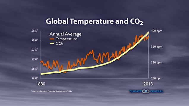
THE EVIDENCE FOR THIS CAUSATION: The evidence for this causation that also serves as the evidence of the effectiveness of the climate action demanded is that since the Industrial Revolution, humans have been burning fossil fuels; and over the same period we find that atmospheric CO2 concentration has been going up. In climate science, this concurrence of emissions and rising atmospheric CO2 over a centennial time scale is taken as evidence of causation in support of the hypothesis that fossil fuel emissions cause atmospheric CO2 concentration to rise; and serves as the rationale for the climate action logic that if we stop burning fossil fuels it will stop the warming. The empirical evidence for this causation is provided as the Airborne Fraction as approximately 50%, that is to say that about half of the fossil fuel emissions is removed by the carbon cycle and the other half remains airborne in the atmosphere.
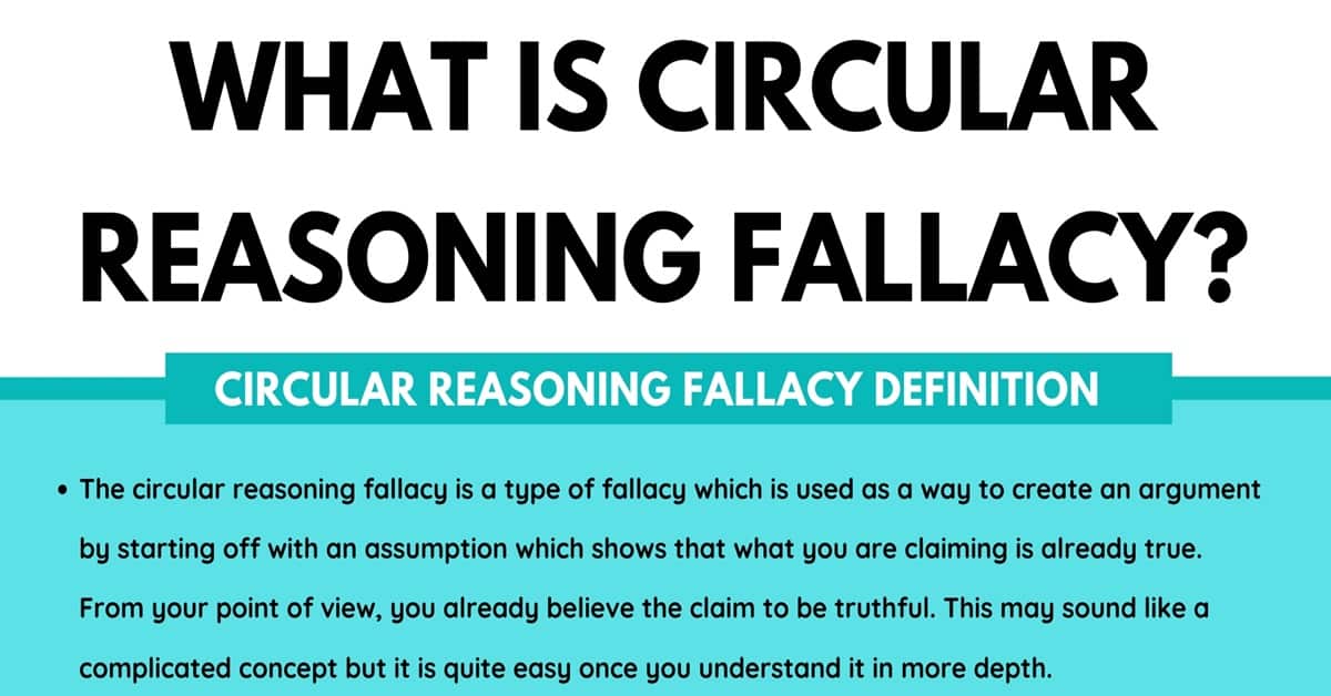
CIRCULAR REASONING IN THIS CAUSATION HYPOTHESIS TEST: In terms of research methodology, what we see here is that the airborne fraction hypothesis was derived from the data and was then tested with the sdame data. This kind of emiprical test is not possible and its results are not credible because the procedure involves circular reasoning. A hyothesis derived from the data cannot be tested with the same data. That kind of hypothesis test suffers from an eextreme form of circular reasoning called the Texas Sharpshooter Fallacy where you shoot first and draw the target circle later. Theefore, the Airborne Fraction argument of climate science is not credible and can be rejected on this basis.

UNCERTAINTY IN THE AIRBORNE FRACTION: As seen in the chart below, although the long term average of the airborne fraction averages out to about 50% or maybe a little higher, the annual mass balance yields a large range for the airborne fraction from 20% to 90%. This variance is defended by the climate science lecture presented above as something that “balances out in the long run” and that it is therefore a statistically valid form of evidence for the causation – that fossil fuel emissions cause atmospheric CO2 to rise. BUT the long run balance is not the issue. In climate science, fossil fuel emissions cause atmospheric CO2 to rise at an annual time scale and therefore this issue must be studied at an annual time scale.

THE AIRBORNE FRACTION: In the lecture above, the climate scientist concedes that there is a mass balance problem with the causation hypothesis that fossil fuel emissions cause atmospheric CO2 concentration to rise. The mass balance shows that the assumed equality of annual fossil fuel emissions and annual rise in atmospheric CO2 is not found in the data. What we find instead is that annual emissions tend to be greater than the annual emissions needed to explain the observed annual change in atmospheric CO2. The explanation for this paradox offered by climate science is that the excess emissions are somehow removed from the atmosphere by carbon cycle flows so that not all the emissions end up in the atmosphere but no mechanism and no empirical evidence for this removal are offered. The portion of annual emissions used to explain the annual change in atmospheric CO2 concentration is called the “Airborne Fraction“.
That the excess annual emissions not explained by annual change in atmospheric CO2 must therefore go somewhere else and if we look through the large carbon cycle flows maybe we can find a way to explain this paradox with the possibility but not the evidence that the missing CO2 goes into carbon cycle flows is a case of circular reasoning and confirmation bias.
These data are interpreted as evidence that about half of the annual emissions stays in the atmosphere {The Airborne Fraction}and causes atmospheric CO2 to rise {to cause warming} and that the other half must therefore be absorbed by nature’s carbon cycle flows to one or more of the sinks in the carbon cycle system.
CIRCULAR REASONING AND CONFIRMATION BIAS: The problem is that this airborne fraction explanation of the emissions mass balance anomaly is a case of circular reasoning and confirmation bias as follows. The airborne fraction was not independently determined from theory but found in the data. A hypothesis was then derived from the data that the excess emissions not explained by the change in atmospheric CO2 are removed by the carbon cycle. This hypothesis was then tested with the same data used to construct the hypothesis. This kind of hypothesis test contains the circular reasoning fallacy. A hypothesis derived from the data cannot be tested with the same data.

PART-3: DETRENDED CORRELATION ANALYSIS OF ANNUAL CHANGES IN MAUNA LOA CO2 CONCENTRATIONS AGAINST ANNUAL FOSSIL FUEL EMISSIONS.
LINK: https://tambonthongchai.com/2020/11/11/annual-changes-in-mlo-co2/


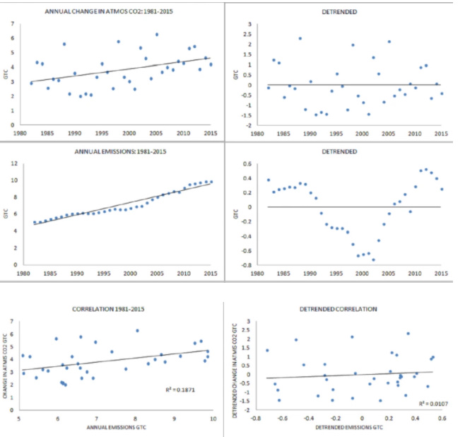
CORRELATION = 0.75


DISCUSSION AND CONCLUSION: THE SOURCE DATA SHOW A STRONG STATISTICALLY SIGNIFICANT CORRELATION OF CORR=0.75 BETWEEN ANNUAL CHANGES IN MLO CO2 AND ANNUAL EMISSIONS. THIS CORRELATION APPEARS TO SUPPORT THE USUAL ASSUMPTION THAT CHANGES IN ATMOSPHERIC CO2 CONCENTRATION ARE CAUSED BY FOSSIL FUEL EMISSIONS AND THAT THEREFORE THESE CHANGES CAN BE MODERATED WITH CLIMATE ACTION TO CONTROL AND REDUCE THE RATE OF WARMING.
HOWEVER, IT IS KNOWN THAT SOURCE DATA CORRELATION BETWEEN TIME SERIES DATA DERIVE FROM TWO SOURCES. THESE ARE (1) SHARED TRENDS WITH NO CAUSATION IMPLICATION AND (2) RESPONSIVENESS AT THE TIME SCALE OF INTEREST. HERE THE TIME SCALE OF INTEREST IS ANNUAL BECAUSE THE THEORY REQUIRES THAT ANNUAL CHANGES IN ATMOSPHERIC CO2 CONCENTRATION ARE CAUSED BY ANNUAL FOSSIL FUEL EMISSIONS. THIS TEST IS MADE BY REMOVING THE SHARED TREND THAT IS KNOWN TO HAVE NO CAUSATION INFORMATION OR IMPLICATION. HERE WE FIND THAT WHEN THE SHARED TREND IS REMOVED THE OBSERVED CORRELATION DISAPPPEARS. THE APPARENT CORRELATION BETWEEN EMISSIONS AND CHANGES IN ATMOSPHERIC CO2 CONCENTRATION IS THUS FOUND TO BE SPURIOUS.
THE DATA FOR ANNUAL FOSSIL FUEL EMISSIONS AND ANNUAL CHANGES IN ATMOSPHERIC CO2 CONCENTRATION DO NOT SHOW THAT FOSSIL FUEL EMISSIONS CAUSE ATMOSPHERIC CO2 CONCENTRATION TO CHANGE. THE FINDING IMPLIES THAT THERE IS NO EMPIRICAL EVIDENCE IN SUPPORT OF THE THEORY OF CLIMATE ACTION. THIS THEORY HOLDS THAT MOVING THE GLOBAL ENERGY INFRASTRUCTURE FROM FOSSIL FUELS TO RENEWABLES WILL MODERATE THE RATE OF INCREASE IN ATMOSPHERIC CO2 AND THEREBY MODERATE THE RATE OF WARMING.

DETRENDED CORRELATION ANALYSIS#2: RESPONSIVENESS OF ATMOSPHERIC COMPOSITION TO FOSSIL FUEL EMISSIONS. LINK: https://tambonthongchai.com/2020/06/14/responsiveness-of-atmospheric-co2-to-fossil-fuel-emissions/
CONCLUSIONS: A key relationship in the theory of anthropogenic global warming (AGW) is that between annual fossil fuel emissions and annual changes in atmospheric CO2. The proposed causation sequence is that annual fossil fuel emissions cause annual changes in atmospheric CO2 which in turn intensifies the atmosphere’s heat trapping property. It is concluded that global warming is due to changes in atmospheric composition attributed to human activity and is therefore a human creation and that therefore we must reduce or eliminate fossil fuel emissions to avoid climate catastrophe (Parmesan, 2003) (Stern, 2007) (IPCC, 2014) (Flannery, 2006) (Allen, 2009) (Gillett, 2013) (Meinshausen, 2009) (Canadell, 2007) (Solomon, 2009) (Stocker, 2013) (Rogelj, 2016). A testable implication of the proposed causation sequence is that annual changes in atmospheric CO2 must be related to annual fossil fuel emissions at an annual time scale. This work is a test of this hypothesis. We find that detrended correlation analysis of annual emissions and annual changes in atmospheric CO2 does not support the anthropogenic global warming hypothesis because no evidence is found that changes in atmospheric CO2 are related to fossil fuel emissions at an annual time scale. These results are consistent with prior works that found no evidence to relate the rate of warming to the rate of emissions (Munshi, The Correlation between Emissions and Warming in the CET, 2017) (Munshi, Long Term Temperature Trends in Daily Station Data: Australia, 2017) (Munshi, Generational Fossil Fuel Emissions and Generational Warming: A Note, 2016) (Munshi, Decadal Fossil Fuel Emissions and Decadal Warming: A Note, 2015) (Munshi, Effective Sample Size of the Cumulative Values of a Time Series, 2016) (Munshi, The Spuriousness of Correlations between Cumulative Values, 2016). The finding raises important questions about the validity of the IPCC carbon budget which apparently overcomes a great uncertainty in much larger natural flows to describe with great precision how flows of annual emissions are distributed to gains in atmospheric and oceanic carbon dioxide (Bopp, 2002) (Chen, 2000) (Davis, 2010) (IPCC, 2014) (McGuire, 2001). These carbon budget conclusions are inconsistent with the findings of this study and are the likely result of insufficient attention to uncertainty, excessive reliance on climate models, and the use of “net flows” (Plattner, 2002) that are likely to be subject to assumptions and circular reasoning (Edwards, 1999) (Ito, 2005) (Munshi, 2015a) (Munshi, 2016) (Munshi, An Empirical Study of Fossil Fuel Emissions and Ocean Acidification, 2015). However, it should be mentioned that though computed values of the “retained fraction” varies from 0.226 to 1.06, the mean value of 0.565 is statistically significant.
DETAILS OF THIS ANALYSIS PROVIDED IN A RELATED POST ON THIS SITE: LINK: https://tambonthongchai.com/2020/06/14/responsiveness-of-atmospheric-co2-to-fossil-fuel-emissions/
DETRENDED CORRELATION ANALYSIS#3: LONGER TIME SCALES. LINK: https://tambonthongchai.com/2018/12/19/co2responsiveness/
TIME SCALES FROM ANNUAL TO 5-YEARS ARE STUDIED. CHART: AIRBORNE FRACTION AT DIFFERENT TIME SCALES.
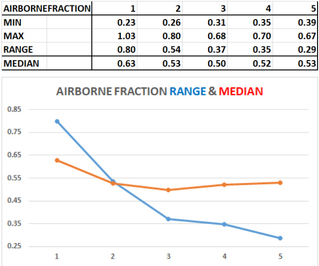
CHART: DETRENDED CORRELATION AT DIFFERENT TIME SCALES

FINDING We conclude that atmospheric composition specifically in relation to the CO2 concentration is not responsive to the rate of fossil fuel emissions. This finding is a serious weakness in the theory of anthropogenic global warming by way of rising atmospheric CO2 attributed to the use of fossil fuels in the industrial economy; and of the “Climate Action proposition of the UN that reducing fossil fuel emissions will moderate the rate of warming by slowing the rise of atmospheric CO2. The finding also establishes that the climate action project of creating Climate Neutral Economies, that is Economies that have no impact on atmospheric CO2, is unnecessary because the global economy is already Climate Neutral.
PART-4: MONTE CARLO SIMULATION OF MIXING CARBON CYCLE FLOWS & FOSSIL FUEL EMISSIONS
The Airborne Fraction issue is studied with Monte Carlo Simulation in two related posts on this site:
SIMULATION#1: :https://tambonthongchai.com/2020/06/10/a-monte-carlo-simulation-of-the-carbon-cycle/
SIMULATION#2: https://tambonthongchai.com/2018/05/31/the-carbon-cycle-measurement-problem/
SIMULATION#1: In SIMULATION#1 we show that the Airborne Fraction anomaly is a serious issue in climate science. As explained above and as seen in the chart below, this critical parameter is not a constant but tends to vary a lot. Specifically, it is not always 50% as claimed in climate science.

The issue in this regard is that to understand the impact of fossil fuel emissions on atmospheric CO2 in terms of carbon cycle flows, we need to be able to measure carbon cycle flows with great precision because these flows are an order of magnitude greater than the relatively small flow of fossil fuel emissions such that even a small random variance in the large carbon cycle flows will make the relatively small fossil fuel emissions undetectable net of the variance in carbon cycle flows.
But the reality is that carbon cycle flows cannot be measured. Their flows can only be inferred from relevant data on the biota and changes in oceanic chemistry etc. Listed below are some IPCC estimates of flow and variance in carbon cycle flows. Other than land use where a mean of 1.1 and a standard deviation of 0.8 pretty much makes that an unknown, the only useful carbon cycle flow data are found for photosynthesis CO2 flow from the atmosphere to the biota. Here, a standard deviation of 8 in a flow estimated to be 123 suggests a ratio where standard deviation is 6.5% of flow. We propose that photosynthesis is a low uncertainty case and therefore to be on the safe side of a Monte Carlo Simulation test of the causation relationship assumed by climate science , we use this percentage standard deviation for all IPCC declared carbon cycle flows to set up a Monte Carlo Simulation of the dynamics of combining the carbon cycle flows and fossil fuel emissions to assess the net impact of fossil fuel emissions on atmospheric composition.
The IPCC list of carbon cycle flows:
Natural: Ocean surface to atmosphere:Mean=78.4,SD=N/A.
Natural: Atmosphere to ocean:surface:Mean=80.0,SD=N/A
Human: Fossil fuel emissions:surface to atmosphere:Mean=7.8,SD=0.6
Human: Land use change:surface to atmosphere:Mean=1.1,SD=0.8
Natural: Photosynthesis:atmosphere to surface:Mean=123.0,SD=8.0
Natural: Respiration/fire:surface to atmosphere:Mean=118.7,SD=N/A
Natural: Freshwater to atmosphere:Mean=1.0,SD=N/A
Natural: Volcanic emissions surface to atmosphere:Mean=0.1,SS =N/A
Natural: Rock weathering:surface to atmosphere:Mean=0.3,SD=N/A
RESULTS OF THE MONTE CARLO SIMULATION#1: THE MONTE CARLO SIMULATION SHOWS THAT THE COMPUTED AIRBORNE FRACTION PROPOSED BY CLIMATE SCIENCE HAS NO INTERPRETATION IN TERMS OF ATMOSPHERIC COMPOSITION BECAUSE IT DOES NOT TAKE UNCERTAINTIES INTO ACCOUNT.
WHEN UNCERTAINTIES ARE TAKEN INTO ACCOUNT NO STATISTICALLY SIGNIFICANT AIRBORNE FRACTION IS FOUND IN THE DATA. THE AIRBORNE FRACTION ARGUMENT PROPOSED BY CLIMATE SCIENCE IS REJECTED ON THE BASIS THAT IT DOES NOT TAKE UNCERTAINTY IN CARBON CYCLE FLOWS ARE INTO ACCOUNT. WHEN THESE UNCERTAINTIES ARE INCLUDED, THE DATA DO NOT SHOW EVIDENCE OF HUMAN CAUSE IN THE OBSERVED CHANGES IN ATMOSPHERIC COMPOSITION.
THEREFORE THERE IS NO EVIDENCE OF HUMAN CAUSE AND NO EVIDENCE FOR THE EFFECTIVENESS OF CLIMATE ACTION.


SIMULATION#2: MONTE CARLO SIMULATION IN REVERESE.
THIS MONTE CARLO SIMULATION IS CARRIED OUT IN REVERESE TO DETERMINE THE MAXIMUM UNCERTANTY IN CARBON CYCLE FLOWS AT WHICH FOSSIL FUEL EMISSIONS CAN STILL BE DETECTED AND MEASURED. LINK: https://tambonthongchai.com/2018/05/31/the-carbon-cycle-measurement-problem/ THIS ANALYSIS IS REPRODUCED BELOW IMMEDIATELY FOLLOWING THE LIST OF CARBON CYCLE FLOWS.
LIST OF CARBON CYCLE FLOWS PROVIDED BY THE IPCC
- Natural: Ocean surface to atmosphere:Mean=78.4,SD=N/A.
- Natural: Atmosphere to ocean:surface:Mean=80.0,SD=N/A
- Human: Fossil fuel emissions:surface to atmosphere:Mean=7.8,SD=0.6
- Human: Land use change:surface to atmosphere:Mean=1.1,SD=0.8
- Natural: Photosynthesis:atmosphere to surface:Mean=123.0,SD=8.0
- Natural: Respiration/fire:surface to atmosphere:Mean=118.7,SD=N/A
- Natural: Freshwater to atmosphere:Mean=1.0,SD=N/A
- Natural: Volcanic emissions surface to atmosphere:Mean=0.1,SS =N/A
- Natural: Rock weathering:surface to atmosphere:Mean=0.3,SD=N/A
- A simple flow accounting of the mean values without consideration of uncertainty shows a net CO2 flow from surface to atmosphere of 4.4 GTC/y. The details of this computation are as follows. In the emissions and atmospheric composition data we find that during the decade 2000-2009 total fossil fuel emissions were 78.1 GTC and that over the same period atmospheric CO2 rose from 369.2 to 387.9 ppm for an increase of 18.7 ppm equivalent to 39.6 GTC in atmospheric CO2 or 4.4 GTC/y. The ratio of the observed increase in atmospheric carbon to emitted carbon is thus =39.6/78.2=0.51. This computation is the source of the claim that the so called “Airborne Fraction” is about 50%; that is to say that about half of the emitted carbon accumulates in the atmosphere on average and the other half is absorbed by the oceans, by photosynthesis, and by terrestrial soil absorption. The Airborne Fraction of AF=50% later had to be made flexible in light of a range of observed values.
- THE CHARTS ABOVE above show that a large range of values of the decadal mean Airborne Fraction of 0
- When uncertainties are not considered, the flow accounting appears to show an exact match of the predicted and computed carbon balance. It is noted, however, that this exact accounting balance is achieved, not with flow measurements, but with estimates of unmeasurable flows constrained by the circular reasoning that assigns flows according to an assumed flow balance.
- However, a very different picture emerges when uncertainties are included in the balance. Published uncertainties for three of the nine flows are available in the IPCC reports. Uncertainty for the other six flows are not known. However, we know that they are large because no known method exists for the direct measurement of these flows. They can only be grossly inferred based on assumptions that exclude geological carbon flows.
- Here, we set up a Monte Carlo simulation to estimate the highest value of the unknown standard deviations of carbon cycle flows at which we can still detect the presence of human emissions within the portfolio of carbon cycle flows. For the purpose of this test we propose that an uncertain flow account is in balance as long as the Null Hypothesis that the sum of the flows is zero cannot be rejected. The alpha error rate for the test is set to a high value of alpha=0.10 to ensure that any reasonable ability to discriminate between the flow account WITH Anthropogenic Emissions from a the flow account WITHOUT Anthropogenic Emissions is taken into evidence that the relatively small fossil fuel emissions can be detected in the presence of much larger and uncertain natural flows. The spreadsheet used in this determination is available for download from an online data archive Data Archive Link .
- In the simulation we assign different levels of uncertainty to the flows for which no uncertainty data are available and test the null hypothesis that the flows balance with anthropogenic emissions (AE) included and again with AE excluded. If the flows balance when AE are included and they don’t balance when AE are excluded then we conclude that the presence of the AE can be detected at that level of uncertainty. However, if the flows balance with and without AE then we conclude that the stochastic flow account is not sensitive to AE at that level of uncertainty because it is unable to detect their presence. If the presence of AE cannot be detected no role for their effect on climate can be deduced from the data at that level of uncertainty in natural flows.
- The balance is computed from the atmospheric perspective as Balance=Input-Output where Input is flow to the atmosphere and Output is flow from the atmosphere. The p-values for hypothesis tests for uncertainties in the natural flows from 1% of mean to 6.5% of mean are presented below both as a tabulation and as a line chart.


- In the tabulation the PCT column shows the assumed percent standard deviation in the natural flows for which no uncertainty information is available. In the”base case”, the blanket statement by the IPCC that the uncertainty is 20% is interpreted to mean that the width of the 95% confidence interval is 20% of the mean and the corresponding standard deviation computed as (20/2)/1.96 is almost identical to that in the 5% (5PC) row. The data in each row shows the p-values of two hypothesis tests labeled as WITH and WITHOUT. The WITH column shows p-values when the AE are included in the balance computation. The WITHOUT column shows the p-values when the AE are left out of the balance computation.
- We use a rather high critical p-value of alpha=0.1 for the test of the null hypothesis that Balance=0 to ensure that any reasonable chance that the effect of fossil fuel emissions can be detected is considered. Balance=0 means that the stochastic flow account is in balance. If the p-value is less than apha we reject the null hypothesis and conclude that the stochastic flow account is not in balance. If we fail to reject the null then we conclude the stochastic flow account is in balance.
- The p-values for WITH and WITHOUT in each row taken together tell us whether the stochastic flow system is sensitive to AE, that is whether the relatively small AE flow can be detected in the context of uncertainty in much larger natural flows. If we fail to reject the null hypothesis that Balance=0 in both WITH and WITHOUT columns, the stochastic flow account balances with and without the AE flows. In these cases the stochastic flow account is not sensitive to AE, that is it is unable to detect the presence of the AE flows. This is true for the five rows in which the uncertainty in natural flows is 3% of mean or higher.
- For the two lower uncertainty levels of 2% and 1% we find that the null hypothesis Balance=0 is not rejected when AE are included (the stochastic flow account is in balance) but rejected when AE are not included (the stochastic flow account is not in balance). Under these uncertainty conditions, the stochastic flow account is sensitive to the presence of AE, that is the flow account can detect the presence of the relatively small AE flows. The chart shows that the crossover uncertainty lies somewhere between 2% and 3% and in fact it is found by trial and error that the crossover occurs at 2.3%.
- These results imply that the IPCC carbon cycle stochastic flow balance is not sensitive to the presence of the relatively low flows from human activity involving fossil fuel emissions and land use change. The large natural flows of the carbon cycle cannot be directly measured and they can only be indirectly inferred. These inferred values contain uncertainties much larger than 2.3% of the mean. It is not possible to carry out a balance of the carbon cycle under these conditions.
- In the case of the conclusion by climate scientists that the observed increase in atmospheric CO2 concentration is caused by fossil fuel emissions, natural flows in the carbon cycle that are an order of magnitude larger than fossil fuel emissions and that cannot be directly measured are inferred with the implicit assumption that the increase in atmospheric CO2 comes from fossil fuel emissions. The flow balance can then be carried out and it does of course show that the increase in atmospheric CO2 derives from fossil fuel emissions The balance presented by the IPCC with inferred flows thus forces an exact balance by way of circular reasoning. Therefore, the IPCC carbon cycle balance does not contain useful information that may be used to ascertain the impact of fossil fuel emissions on the carbon cycle or on the climate system.
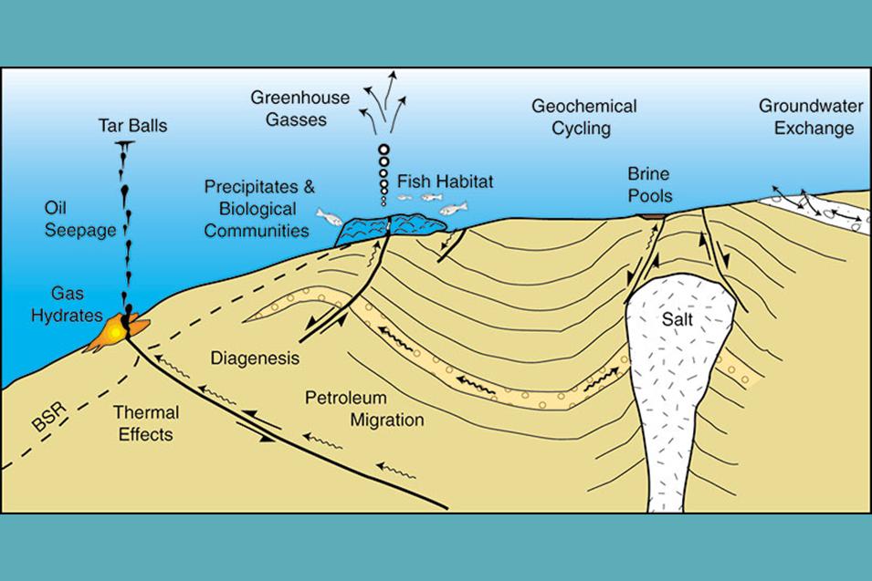
- A rationale for the inability to relate changes in atmospheric CO2 to fossil fuel emissions is described by Geologist James Edward Kamis in terms of natural geological emissions due to plate tectonics [LINK] . The essential argument is that, in the context of significant geological flows of carbon dioxide and other carbon based compounds, it is a form of circular reasoning to describe changes in atmospheric CO2 only in terms of human activity. It is shown in a related post, that in the context of large uncertainties in natural flows, changes in atmospheric CO2 is not responsive to the rate of emissions [LINK] .
- Circular reasoning in this case can be described in terms of the “Assume a spherical cow” fallacy [LINK] which refers to the use of simplifying assumptions needed to solve a problem that change the context of the problem so that the solution no longer answers the original research question. WE CONCLUDE THAT THE UNCERTAINTY IN CARBON CYCLE FLOWS ARE TOO LARGE TO MEASURE THE EFFECT OF RELATIVELY SMALL FLOWS OF FOSSIL FUEL EMISSIONS ON ATMOSPHERIC COMPOSITION.
CONCLUSION
DETRENDED CORRELATION ANALYSIS AND MONTE CARLO SIMULATION ARE USED TO STUDY TO RESPONSIVENESS OF ATMOSPHERIC COMPOSITION TO FOSSIL FUEL EMISSIONS. NO EVIDENCE IS FOUND TO SUPPORT THE ASSUMED CAUSATION IN CLIMATE SCIENCE WHERE THE OBSERVED RISE IN ATMOSPHERIC CO2 CONCENTRATION IS ATTRIBUTED TO FOSSIL FUEL EMISSIONS. THE FINDINGS PRESENTED ABOVE IMPLY THAT THE AIRBORNE FRACTION IS A CREATION OF CIRCULAR REASONING AND CONFRMATION BIAS.


IT IS NOTED IN A RELATED POST THAT GEOLOGICAL FLOWS OF CARBON AND CO2 ARE EXCLUDED IN THE STUDY OF THE RISE IN ATMOSPHERIC CO2 SINCE PRE-INDUSTRIAL WHERE THE INDUSTRIAL CAUSE IS SUBSUMED INTO THE STUDY METHODOLOGY. LINK: https://tambonthongchai.com/2019/08/27/carbonflows/ With respect to the argument that the absence of 13C and 14C isotopes identify fossil fuel carbon it should be noted that fossil fuel carbon and geological carbon cannot be distinguished from each other on this basis because neither contains these carbon isotopes.
RELATED POST ON CONFIRMATION BIAS IN SUPERSTITION. LINK: https://tambonthongchai.com/2018/08/03/confirmationbias/