
Why Models Can’t Predict Temperature: A History Of Failure
By Christopher Monckton of Brenchley | May 9, 2021
This is a long and technical posting. If you don’t want to read it, don’t whine.
The first scientist to attempt to predict eventual warming by doubled CO2, known to the crystal-ball gazers as equilibrium doubled-CO2 sensitivity (ECS), was the Nobel laureate Svante Arrhenius, a chemist, in 1896. He had recently lost his beloved wife. To keep his mind occupied during the long Nordic winter, he carried out some 10,000 spectral-line calculations by hand and concluded that ECS was about 5 C°.
However, he had relied upon what turned out to be defective lunar spectral data. Realizing this, he recalculated ten years later and, in 1906, published a second paper, in which he did what climate “scientists” refuse to do today: he recanted his first paper and published a revised estimate, this time in German, which true-believing Thermageddonites seldom cite:
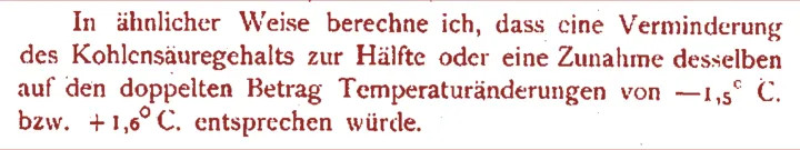
His corrected calculation, published in the then newly-founded Journal of the Royal Nobel Institute, suggested 1.6 C° ECS, including the water-vapor feedback response.
Guy Stewart Callendar, a British steam engineer, published his own calculation in 1938, and presented his result before the Royal Society (the Society’s subsequent discussion is well worth reading). He, too, predicted 1.6 C° ECS, as the dotted lines I have added to his graph demonstrate:

Then there was a sudden jump in predicted ECS. Plass (1956) predicted 3.6 C° ECS. Möller (1963) predicted a direct or reference doubled-CO2 sensitivity (RCS) of 1.5 C°, rising to as much as 9.6 C° if relative humidity did not change. He added an important rider: “…the variation in the radiation budget from a changed CO2 concentration can be compensated for completely without any variation in the surface temperature when the cloudiness is increased by +0.006.” Unsurprisingly, he concluded that “the theory that climatic variations are effected by variations in the CO2 content becomes very questionable.”
Manabe & Wetherald (1975), using an early radiative-convective model, predicted 2.3 C° ECS. Hansen (1981) gave a midrange estimate of 2.8 C° ECS. In 1984 he returned to the subject, and, for the first time, introduced feedback formulism from control theory, the study of feedback processes in dynamical systems (systems that change their state over time). He predicted 1.2 C° RCS and 4 C° ECS, implying a feedback fraction 0.7.
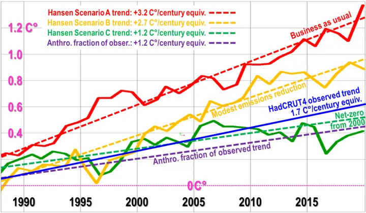
In 1988, in now-notorious testimony before the U.S. Senate during a June so hot that nothing like it has been experienced in Washington DC since, he predicted 3.2 C° per century (broadly equivalent to ECS) on a business-as-usual scenario (and it is the business-as-usual scenario that has happened since), but anthropogenic warming is little more than a third of his predicted business-as-usual rate:
In 1988 the late Michael Schlesinger returned to the subject of temperature feedback, and found that in a typical general-circulation model the feedback fraction – i.e., the fraction of equilibrium sensitivity contributed by feedback response – was an absurdly elevated 0.71, implying a system-gain factor (the ratio of equilibrium sensitivity after feedback to reference sensitivity before it) of 3.5 and thus, assuming 1.05 RCS, an ECS of 3.6 C°.
Gregory et al. (2002) introduced a simplified method of deriving ECS using an energy-balance method. Energy-balance methods had been around for some time, but it was not until the early 2000s that satellite and ocean data became reliable enough and comprehensive enough to use this simple method. Gregory generated a probability distribution, strongly right-skewed (for a reason that will become apparent later), with a midrange estimate of 2 C° ECS:

Gregory’s result has been followed by many subsequent papers using the energy-balance method. Most of them find ECS to be 1.5-2 C°, one-third to one-half of the 3.7-4 C° midrange that the current general-circulation models predict.
In 2010 Lacis et al., adhering to the GCMs’ method, wrote:
“For the doubled-CO2 irradiance forcing, … for which the direct no-feedback response of the global surface temperature [is] 1.2 C° …, the ~4 C° surface warming implies [a] … [system-gain factor] of 3.3. … “
Lacis et al. went on to explain why they thought there would be so large a system-gain factor, which implies a feedback fraction of 0.7:
Noncondensing greenhouse gases, which account for 25% of the total terrestrial greenhouse effect, … provide the stable temperature structure that sustains the current levels of atmospheric water vapor and clouds via feedback processes that account for the remaining 75% of the greenhouse effect.
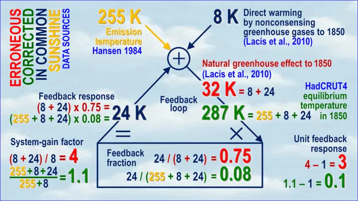
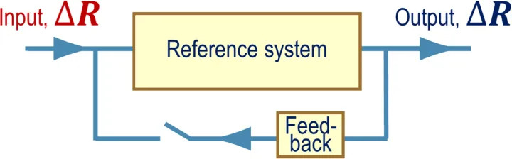
Unfortunately, the above passage explicitly perpetrates an extraordinary error, universal throughout climatology, which is the reason why modelers expect – and hence their models predict – far larger warming than the direct and simple energy-balance method would suggest. The simple block diagram below will demonstrate the error by comparing erroneous (red) against corrected (green) values all round the loop:
Let us walk round the feedback loop for the preindustrial era. We examine the preindustrial era because when modelers were first trying to estimate the influence of the water-vapor and other feedbacks, none of which can be directly and reliably quantified by measurement or observation, they began with the preindustrial era.
For instance, Hansen (1984) says:
“… this requirement of energy balance yields [emission temperature] of about 255 K. … the surface temperature is about 288 K, 33 K warmer than emission temperature. … The equilibrium global mean warming of the surface air is about 4 C° … This corresponds to a [system-gain factor] 3-4, since the no-feedback temperature change required to restore radiative equilibrium with space is 1.2-1.3 C°.
First, let us loop the loop climatology’s way. The direct warming by preindustrial noncondensing greenhouse gases (the condensing gas water vapor is treated as a feedback) is about 8 K, but the total natural greenhouse effect, the difference between the 255 K emission temperature and the 287 K equilibrium global mean surface temperature in 1850 is 32 K. Therefore, climatology’s system-gain factor is 32 / 8, or 4, so that its imagined feedback fraction is 1 – 1/4, or 0.75 – again absurdly high. Thus, 1 K RCS would become 4 K ECS.
Now let us loop the loop control theory’s way, first proven by Black (1934) at Bell Labs in New York, and long and conclusively verified in practice. One must not only input the preindustrial reference sensitivity to noncondensing greenhouse gases into the loop via the summative input/output node at the apex of the loop: one must also input the 255 K emission temperature (yellow), which is known as the input signal (the clue is in the name).
It’s the Sun, stupid!
Then the output from the loop is no longer merely the 32 K natural greenhouse effect: it is the 287 K equilibrium global mean surface temperature in 1850. The system-gain factor is then 287 / (255 + 8), or 1.09, less than a third of climatology’s estimate. The feedback fraction is 1 – 1 / 1.09, or 0.08, less by an order of magnitude than climatology’s estimate.
Therefore, contrary to what Hansen, Schlesinger, Lacis and many others imagine, there is no good reason in the preindustrial data to expect that feedback on Earth is unique in the solar system for its magnitude, or that ECS will be anything like the imagined three or four times RCS.
As can be seen from the quotation from Lacis et al., climatology in fact assumes that the system-gain factor in the industrial era will be about the same as that for the preindustrial era. Therefore, the usual argument against the corrected preindustrial calculation – that it does not allow for inconstancy of the unit feedback response with temperature – is not relevant.
Furthermore, a simple energy-balance calculation of ECS using current mainstream industrial-era data in a method entirely distinct from the preindustrial analysis and not dependent upon it in any way comes to the same answer as the corrected preindustrial method: a negligible contribution from feedback response. Accordingly, unit feedback response is approximately constant with temperature, and ECS is little more than the 1.05 K RCS.
Why, then, do the models get their predictions so wrong? In the medium term (top of the diagram below), midrange projected anthropogenic medium-term warming per century equivalent was 3.4 K as predicted by IPCC in 1990, but observed warming was only 1.65 K, of which only 70% (Wu et al. 2019), or 1.15 K, was anthropogenic. IPCC’s prediction was thus about thrice subsequently-observation, in line with the error but not with reality.
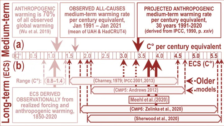
Since the currently-estimated doubled-CO2 radiative forcing is about the same as predicted radiative forcing from all anthropogenic sources over the 21st century, one can observe in the latest generation of models much the same threefold exaggeration compared with the 1.1 K ECS derivable from current climate data (bottom half of the above diagram), including real-world warming and radiative imbalance, via the energy-balance method.
The error of neglecting the large feedback response to emission temperature, and of thus effectively adding it to, and miscounting it as though it were part of, the actually minuscule feedback response to direct greenhouse-gas warming, is elementary and grave. Yet it seems to be universal throughout climatology. Here are just a few statements of it:
The American Meteorological Society (AMS, 2000) uses a definition of feedback that likewise overlooks feedback response to the initial state –
“A sequence of interactions that determines the response of a system to an initial perturbation”.
Soden & Held (2006) also talk of feedbacks responding solely to perturbations, but not also to emission temperature–
“Climate models exhibit a large range of sensitivities in response to increased greenhouse gases due to differences in feedback processes that amplify or dampen the initial radiative perturbation.”
Sir John Houghton (2006), then chairman of IPCC’s climate-science working party, was asked why IPCC expected a large anthropogenic warming. Sir John replied that, since preindustrial feedback response accounted for three-quarters of the natural greenhouse effect, so that the preindustrial system-gain factor was , and one would thus expect a system-gain factor of
or
today.
IPCC (2007, ch. 6.1, p. 354) again overlooks the large feedback response to the 255 K emission temperature:
“For different types of perturbations, the relative magnitudes of the feedbacks can vary substantially.”
Roe (2009), like Schlesinger (1988), shows a feedback block diagram with a perturbation ∆R as the only input, and no contribution to feedback response by emission temperature –
Yoshimori et al. (2009) say:
“The conceptually simplest definition of climate feedback is the processes that result from surface temperature changes, and that result in net radiation changes at the top of the atmosphere (TOA) and consequent surface temperature changes.”
Lacis et al. (2010) repeat the error and explicitly quantify its effect, defining temperature feedback as responding only to changes in the concentration of the preindustrial noncondensing greenhouse gases, but not also to emission temperature itself, consequently imagining that ECS will be times the
degree direct warming by those gases:
“This allows an empirical determination of the climate feedback factor [the system-gain factor] as the ratio of the total global flux changeto the flux change that is attributable to the radiative forcing due to the noncondensing greenhouse gases. This empirical determination … implies that Earth’s climate system operates with strong positive feedback that arises from the forcing-induced changes of the condensable species. … noncondensing greenhouse gases constitute the key 25% of the radiative forcing that supports and sustains the entire terrestrial greenhouse effect, the remaining 75% coming as fast feedback contributions from the water vapor and clouds.”
Schmidt et al. (2010) find the equilibrium doubled-CO2 radiative forcing to be five times the direct forcing:
“At the doubled-CO2 equilibrium, the global mean increase in … the total greenhouse effect is ~20 W m-2, significantly larger than the ≥ 3initial forcing and demonstrating the overall effect of the long-wave feedbacks is positive (in this model).”
IPCC (2013, p. 1450) defines what Bates (2016) calls “sensitivity-altering feedback” as responding solely to perturbations, which are mentioned five times, but not also to the input signal, emission temperature:
“Climate feedback: An interaction in which a perturbation in one climate quantity causes a change in a second, and the change in the second quantity ultimately leads to an additional change in the first. A negative feedback is one in which the initial perturbation is weakened by the changes it causes; a positive feedback is one in which the initial perturbation is enhanced … the climate quantity that is perturbed is the global mean surface temperature, which in turn causes changes in the global radiation budget. … the initial perturbation can … be externally forced or arise as part of internal variability.”
Knutti & Rugenstein (2015) likewise make no mention of base feedback response:
“The degree of imbalance at some time following a perturbation can be ascribed to the temperature response itself and changes induced by the temperature response, called feedbacks.”
Dufresne & St.-Lu (2015) say:
“The response of the various climatic processes to climate change can amplify (positive feedback) or damp (negative feedback) the initial temperature perturbation.”
Heinze et al. (2019) say:
“The climate system reacts to changes in forcing through a response. This response can be amplified or damped through positive or negative feedbacks.”
Sherwood et al. 2020 also neglect emission temperature as the primary driver of feedback response –
“The responses of these [climate system] constituents to warming are termed feedback. The constituents, including atmospheric temperature, water vapor, clouds, and surface ice and snow, are controlled by processes such as radiation, turbulence, condensation, and others. The CO2 radiative forcing and climate feedback may also depend on chemical and biological processes.”
The effect of the error is drastic indeed. The system-gain factor and thus ECS is overstated threefold to fourfold; the feedback fraction is overestimated tenfold; and the unit feedback response (i.e., the feedback response per degree of direct warming before accounting for feedback) is overstated 30-fold at midrange and 100-fold at the upper bound of the models’ predictions.
The error can be very simply understood by looking at how climatology and control theory would calculate the system-gain factor based on preindustrial data:
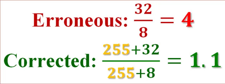
Since RCS is little more than 1 K, ECS once the sunshine temperature of 255 K has been added to climatology’s numerator and denominator to calm things down, is little more than the system-gain factor. And that is the end of the “climate emergency”. It was all a mistake.
Of course, the models do not incorporate feedback formulism directly. Feedbacks are diagnosed ex post facto from their outputs. Recently an eminent skeptical climatologist, looking at our result, said we ought to have realized from the discrepancy between the models’ estimates of ECS and our own that we must be wrong, because the models were a perfect representation of the climate.
It is certainly proving no less difficult to explain the control-theory error to skeptics than it is to the totalitarian faction that profiteers so mightily by the error. Here, then, is how our distinguished co-author, a leading professor of control theory, puts it:
Natural quantities are what they are. To define a quantity as the sum of a base signal and its perturbation is a model created by the observer. If the base signal – analogous to the input signal in an electronic circuit – is chosen arbitrarily, the perturbation (the difference between the arbitrarily-chosen baseline and the quantity that is the sum of the baseline and the perturbation) ceases to be a real, physical quantity: it is merely an artefact of a construct that randomly divides a physical quantity into multiple components. However, the real system does not care about the models created by its observer. This can easily be demonstrated by the most important feedback loop of all, the water vapour feedback, where warming causes water to evaporate and the resulting water vapour, a greenhouse gas, forces additional warming.
Climatology defines feedback in such a way that only the perturbation – but not also the base signal, emission temperature – triggers feedback response. The implication is that in climatologists’ view of the climate the sunshine does not evaporate any water. In their models, the 1363.5 W m-2 total solar irradiance does not evaporate a single molecule of water, while the warming caused by just 25 W m-2 of preindustrial forcing by noncondensing greenhouse gases is solely responsible for all the naturally-occurring evaporation of water on earth. This is obvious nonsense. Water cares neither about the source of the heat that evaporates it nor about climatology’s erroneous definitions of feedback. In climatology’s model, the water vapour feedback would cease to work if all the greenhouse gases were removed from the atmosphere. The Sun, through emission temperature, would not evaporate a single molecule of water, because by climatologists’ definition sunshine does not evaporate water.
Heat is the same physical quantity, no matter what the source of the heat is. The state of a system can be described by the heat energy it contains, no matter what the source of the heat is. Temperature-induced feedbacks are triggered by various sources of heat. The Sun is the largest such source. Heat originating from solar irradiance follows precisely the same natural laws as heat originating from the greenhouse effect does. All that counts in analysing the behaviour of a physical system is the total heat content, not its original source or sources.
Climatology’s models fail to reflect this fact. A model of a natural system must reflect that system’s inner workings, which may not be defined away by any “consensus”. The benchmark for a good model of a real system is not “consensus” but objective reality. The operation of a feedback amplifier in a dynamical system such as the climate (a dynamical system being one that changes its state over time) is long proven theoretically and repeatedly demonstrated in real-world applications, such as control systems for power stations, space shuttles, the flies on the scape-shafts of church-tower clocks, the governors on steam engines, and increased specific humidity with warmer weather in the climate, and the systems that got us to the Moon.
Every control theorist to whom we have shown our results has gotten the point at once. Every climatologist – skeptical as well as Thermageddonite – has wriggled uncomfortably. For control theory is right outside climatology’s skill-set and comfort zone.
So let us end with an examination of why it is that the “perfect” models are in reality, and formally, altogether incapable of telling us anything useful whatsoever about how much global warming our industries and enterprises may cause.
The models attempt to solve the Navier-Stokes equations using computational fluid dynamics for cells typically 100 km x 100 km x 1 km, in a series of time-steps. Given the surface area of of the Earth and the depth of the troposphere, the equations must be solved over and over again, time-step after time-step, for each of about half a million such cells – in each of which many of the relevant processes, such as Svensmark nucleation, take place at sub-grid scale and are not captured by the models at all.
Now the Navier-Stokes equations are notoriously refractory partial differential equations: so intractable, in fact, that no solutions in closed form have yet been found. They can only be solved numerically and, precisely because no closed-form solutions are available, one cannot be sure that the numerical solutions do not contain errors.
Here are the Navier-Stokes equations:

So troublesome are these equations, and so useful would it be if they could be made more tractable, that the Clay Mathematics Institute is offering a $1 million Millennium Prize to the first person to demonstrate the existence and smoothness (i.e., continuity) of real Navier-Stokes solutions in three dimensions.
There is a further grave difficulty with models that proceed in a series of time-steps. As Pat Frank first pointed out in a landmark paper of great ingenuity and perception two years ago – a paper, incidentally, that has not yet met with any peer-reviewed refutation – propagation of uncertainty through the models’ time-steps renders them formally incapable of telling us anything whatsoever about how much or how little global warming we may cause. Whatever other uses the models may have, their global-warming predictions are mere guesswork, and are wholly valueless.
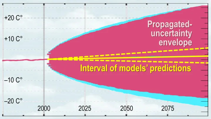
One problem is that the uncertainties in key variables are so much larger than the tiny mean anthropogenic signal of less than 0.04 Watts per square meter per year. For instance, the low-cloud fraction is subject to an annual uncertainty of 4 Watts per square meter (derived by averaging over 20 years). Since propagation of uncertainty proceeds in quadrature, this one uncertainty propagates so as to establish on its own an uncertainty envelope of ±15 to ±20 C° over a century. And there are many, many such uncertainties.
Therefore, any centennial-scale prediction falling within that envelope of uncertainty is nothing more than a guess plucked out of the air. Here is what the uncertainty propagation of this one variable in just one model looks like. The entire interval of CMIP6 ECS projections falls well within the uncertainty envelope and, therefore, tells us nothing – nothing whatsoever – about how much warming we may cause.
Pat has had the same difficulty as we have had in convincing skeptics and Thermageddonites alike that he is correct. When I first saw him give a first-class talk on this subject, at the World Federation of Scientists’ meeting at Erice in Sicily in 2016, he was howled down by scientists on both sides in a scandalously malevolent and ignorant manner reminiscent of the gross mistreatment of Henrik Svensmark by the profiteering brutes at the once-distinguished Royal Society some years ago.
Here are just some of the nonsensical responses Pat Frank has had to deal with over the past couple of years since publication, and before that from reviewers at several journals that were simply not willing to publish so ground-breaking a result:
Nearly all the reviewers of Dr Frank’s paper a) did not know the distinction between accuracy and precision; b) did not understand that a temperature uncertainty is not a physical temperature interval; c) did not realize that deriving an uncertainty to condition a projected temperature does not imply that the model itself oscillates between icehouse and greenhouse climate predictions [an actual objection from a reviewer]; d) treated propagation of uncertainty, a standard statistical method, as an alien concept; e) did not understand the purpose or significance of a calibration experiment; f) did not understand the concept of instrumental or model resolution or their empirical limits; g) did not understand physical uncertainty analysis at all; h) did not even appreciate that ±n is not the same as +n; i) did not realize that the ± 4 W m–2 uncertainty in cloud forcing was an annual mean derived from 20 years’ data; j) did not understand the difference between base-state error, spatial root-mean-square error and global mean net error; k) did not realize that taking the mean of uncertainties cancels the signs of the errors, concealing the true extent of the uncertainty; l) did not appreciate that climate modellers’ habit of taking differences against a base state does not subtract away the uncertainty; m) imagined that a simulation error in tropospheric heat content would not produce a mistaken air temperature; did not understand that the low-cloud-fraction uncertainty on which the analysis was based was not a base-state uncertainty, nor a constant error, nor a time-invariant error; n) imagined that the allegedly correct 1988-2020 temperature projection by Hansen (1988) invalidated the analysis.
Bah! We have had to endure the same sort of nonsense, and for the same reason: climatologists are insufficiently familiar with relevant fields of mathematics, physics and economics outside their own narrow and too often sullenly narrow-minded specialism, and are most unwilling to learn.
The bottom line is that climatology is simply wrong about the magnitude of future global warming. No government should pay the slightest attention to anything it says.